XGBoost Multi-Output Regression: One Tree, Many Targets

Most gradient boosting examples have one target. You predict a house price, a probability, a demand value, or some other single number. Real datasets are often less tidy. The same house may have a sale price and a time on market. A sensor can produce temperature and pressure readings. A financial instrument can have returns measured over several different horizons. The input features are the same, but there are several things you want to predict.

XGBoost supports multi-output regression in two different ways. The default strategy effectively builds a separate tree for every target on each boosting round. The alternative, called multi_output_tree, builds one shared tree whose leaves contain a vector of values, one value for each target. That second approach is usually called a vector leaf.

The interesting question is not only whether it is smaller or faster. Sharing a tree forces the targets to use the same split structure, which changes what the model can learn. In this article, I will first show how the two strategies differ, then look at when shared trees should help, and finally test them on a difficult real-world dataset from Numerai. The experiment uses 2.7 million rows, 780 features, and two related stock-return targets.

The default: one model per target

XGBoost has accepted multi-output labels since version 1.6. If y contains several columns, you can pass it directly to XGBRegressor:

import numpy as np
import xgboost as xgb

X = np.random.rand(1000, 20)
y = np.random.rand(1000, 3)

model = xgb.XGBRegressor(tree_method="hist")
model.fit(X, y)

model.predict(X).shape

The output shape is (1000, 3). So from the outside, this already looks like one model that predicts three values. Internally, the default strategy is closer to training one model per target. Each boosting round adds one tree for each output. With three targets, one boosting round creates three trees. After 500 rounds, the model contains 1,500 trees. Those targets do not share the tree structure. Target 1 can split on one feature, while target 2 can choose something completely different. This is similar in spirit to scikit-learn's MultiOutputRegressor, although XGBoost can reuse the same input data matrix.

What is a vector leaf?

A normal regression tree stores one number in each leaf.

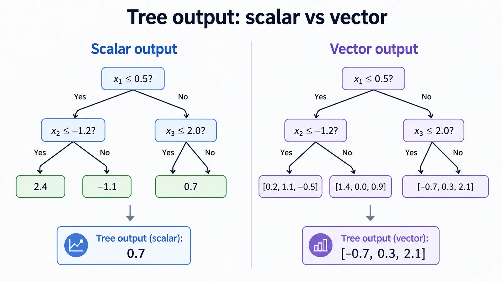
Imagine three targets and a single boosting round. With the default strategy, we might get three separate trees:

tree A, target 1       tree B, target 2       tree C, target 3

f7 < 0.4?              f2 < 0.9?              f7 < 0.35?
 /     \                /     \                /      \
0.12  -0.03            0.44   0.01            0.09   -0.05

Each target is free to choose its own splits.

A vector-leaf model instead builds one shared tree:

one shared tree

f7 < 0.4?
 /              \
[0.12, 0.41, 0.10]   [-0.03, 0.02, -0.06]

The split is shared, but each leaf contains a different update for every target. So three trees become one. The targets agree on the partition of the feature space, while still receiving different predictions inside each leaf. You enable this behavior with one parameter:

model = xgb.XGBRegressor(
    tree_method="hist",
    multi_strategy="multi_output_tree",
)

model.fit(X, y)

The default value is one_output_per_tree. For larger datasets, the native XGBoost API is also available:

dtrain = xgb.QuantileDMatrix(X, label=y)

params = {
    "objective": "reg:squarederror",
    "tree_method": "hist",
    "multi_strategy": "multi_output_tree",
}

booster = xgb.train(
    params,
    dtrain,
    num_boost_round=500,
)

pred = booster.inplace_predict(X)

The prediction still has shape:

(n_rows, n_targets)

There are some constraints to know. Vector leaves use the hist tree method, the feature is still marked experimental, gblinear is not supported, and the documentation currently focuses on the Python package.

A short version history

The multi_output_tree parameter is not brand new, but its implementation has changed considerably over time.

Version	Date	What changed
1.6	2022	Multi-output regression and multi-label classification accepted, using one model per target
2.0	Sep 2023	Vector leaves prototyped for CPU hist through multi_strategy
3.1	Sep 2025	Intercept stored as a vector for multi-output models, groundwork for vector leaf
3.2	Feb 2026	Reduced-gradient training added for large target counts
3.4	Aug 2026	Vector-leaf support for hist became feature-complete and moved to experimental

The practical difference is important. The parameter existed in earlier versions, but many capabilities were missing. With XGBoost 3.4.1, released ten days after 3.4.0, the hist implementation covers CPU and CUDA training, categorical splits, and reduced-gradient training. That is the version I used for the experiment in this article. The XGBoost team also published their own vector-leaf demo results on multiclass classification. So if you tried multi_output_tree a few years ago and found it too limited, it is worth testing again with a recent release.

The important idea: partition compatibility

It is tempting to think that shared trees are useful whenever the targets are correlated. That is not quite the right condition. What matters more is whether the targets benefit from similar partitions of the feature space. The XGBoost authors call this partition compatibility.

Suppose two targets are both influenced by the same feature:

feature_7 < 0.4

The actual target values may not be strongly correlated, but this split could still be useful for both of them. The opposite can also happen. Two target values may be strongly correlated overall, but one target wants to split on feature 7 while the other needs feature 22. Forcing both through the same tree structure can then hurt. This distinction is important because sharing a tree is a structural assumption. You are saying that the targets can usefully divide the feature space in similar ways.

When that assumption is reasonable, vector leaves can offer several advantages.

The first is model size. Instead of adding one tree per target on every boosting round, the model adds one shared tree. The benefit grows with the number of outputs. In the XGBoost team's tests with 32 outputs, the vector model was roughly one ninth of the serialized size and also showed faster training and prediction.

The second possible advantage is regularization. A split has to be useful across the targets rather than being selected only because it happens to improve one output. In experiments with added noise features, scalar models spent more split gain on irrelevant features than vector models.

The third is that shared structure can act as a prior. If several targets are different views of the same underlying process, asking them to share partitions may be exactly the restriction you want.

The trade-off is flexibility. If the targets genuinely require different splits, separate trees have more freedom.

Why financial data often has several targets

Financial datasets are a natural place to test multi-output models because there is rarely only one definition of a future return. The same instrument can be evaluated over 20 days, 60 days, or another horizon. Returns can be raw or neutralized against sectors, countries, or known risk factors. This creates several labels for exactly the same feature rows.

Public machine-learning competitions often expose this structure. Numerai provides families of targets for the same observations. Its documentation describes the auxiliary targets as stock-specific returns that differ in what gets residualized and over what horizon, and notes that a model trained on an auxiliary target sometimes outperforms one trained on the main target. In my experiment, I used two targets from the 60-day family.

Jane Street competitions have also included multiple response variables. The 2024 Real-Time Market Data Forecasting competition had nine responders, even though only one was directly scored. The 2021 Market Prediction competition similarly provided resp together with resp_1 through resp_4.

The interesting part is that auxiliary targets provide additional supervision without requiring additional feature rows. A common approach is to train only on the target that will ultimately be scored and ignore the others. A more sophisticated one is to train a model per target and blend the predictions, which is what Numerai's own target ensemble notebook demonstrates. Vector leaves give us a third option: let several targets participate in deciding the tree structure itself. The experiment below tests all three.

The experiment

I wanted the comparison to be as simple as possible, so there is no parameter tuning, no early stopping, no ensembling search, and only one random seed. The dataset is Numerai v5.3 using the medium feature set, which contains 780 features. Rows with either target missing were removed so every candidate model saw exactly the same samples. The training set contains 2,746,268 rows covering eras 1 through 574. I then skipped eras 575 through 586 as an embargo because the 60-day target overlaps the end of the training period. I used 12 eras, matching the 60-business-day horizon. Numerai's documentation suggests 16 purge eras for 60-day targets, so this is slightly shorter. It applies identically to every candidate, so it does not favour one strategy over another. Validation starts at era 587 and continues through era 1221, giving 635 validation eras.

The primary target is:

target_ender_60

and the second target is:

target_tyler_60

All models use the same basic parameters:

params = {
    "objective": "reg:squarederror",
    "tree_method": "hist",
    "device": "cpu",
    "learning_rate": 0.05,
    "max_depth": 5,
    "max_bin": 64,
    "min_child_weight": 20,
    "subsample": 0.8,
    "colsample_bytree": 0.2,
    "seed": 42,
}

NUM_BOOST_ROUND = 500

I compared four candidates, all evaluated against Ender60.

1. The first is a normal scalar model trained directly on Ender60.

2. The second is another scalar model trained on Tyler60, but evaluated against Ender60. This tells us how useful the partner target is by itself.

3. The third candidate is a simple 50/50 rank average of the two scalar predictions.

4. The fourth is a vector-leaf model trained on Ender60 and Tyler60 together. For evaluation, I use only its Ender output.

The third candidate is an important control. If using two targets helps, the obvious question is whether we could simply train two independent models and average their predictions afterwards. The vector model needs to beat that idea, not just a single-target baseline.

Metrics

I used two Numerai metrics. The first is CORR60, which measures rank correlation with the target after Numerai's standard transformations. The second is BMC60, which measures what remains after projecting the prediction away from Numerai's benchmark model. BMC is especially interesting because it asks whether the model is adding something that the benchmark does not already contain. A model can have reasonable raw correlation while contributing very little new information relative to the benchmark.

Choosing the second target

Before training, I ranked the other 60-day targets by their Spearman correlation with Ender60.

Some examples:

Target	Spearman with Ender60
tyler_60	0.6637
agnes_60	0.6638
alpha_60	0.6935
...	...
teager2b_60	0.7849
jasper_60	0.7901

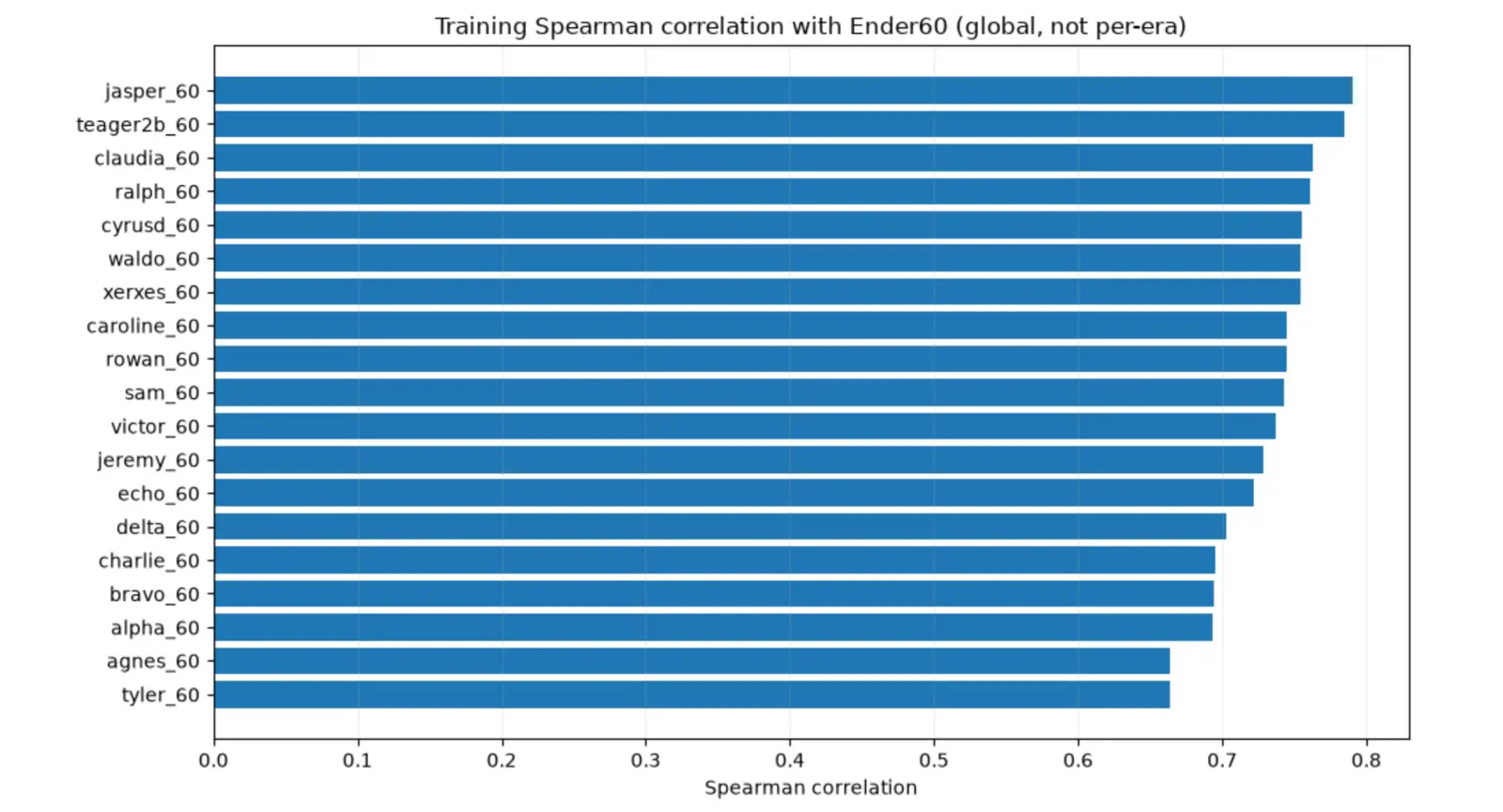
Tyler is at the bottom of this list. It is the least correlated 60-day target in the set. I chose it deliberately. If I paired Ender with something like Jasper at 0.79 correlation, the two targets would already be quite similar. A positive result would make it harder to tell whether vector leaves were benefiting from shared partitions or simply from receiving almost the same target twice. Tyler makes the test more interesting. If partition compatibility is genuinely different from target correlation, a less correlated partner can still be useful.

Results

Here are the mean per-era metrics across 635 validation eras:

Candidate	CORR60	BMC60
Scalar Ender	0.028379	0.001126
Scalar Tyler	0.022761	-0.001367
Scalar Ender + Tyler, 50/50	0.028103	-0.000039
Vector (Ender, Tyler), Ender head	0.028705	0.001142

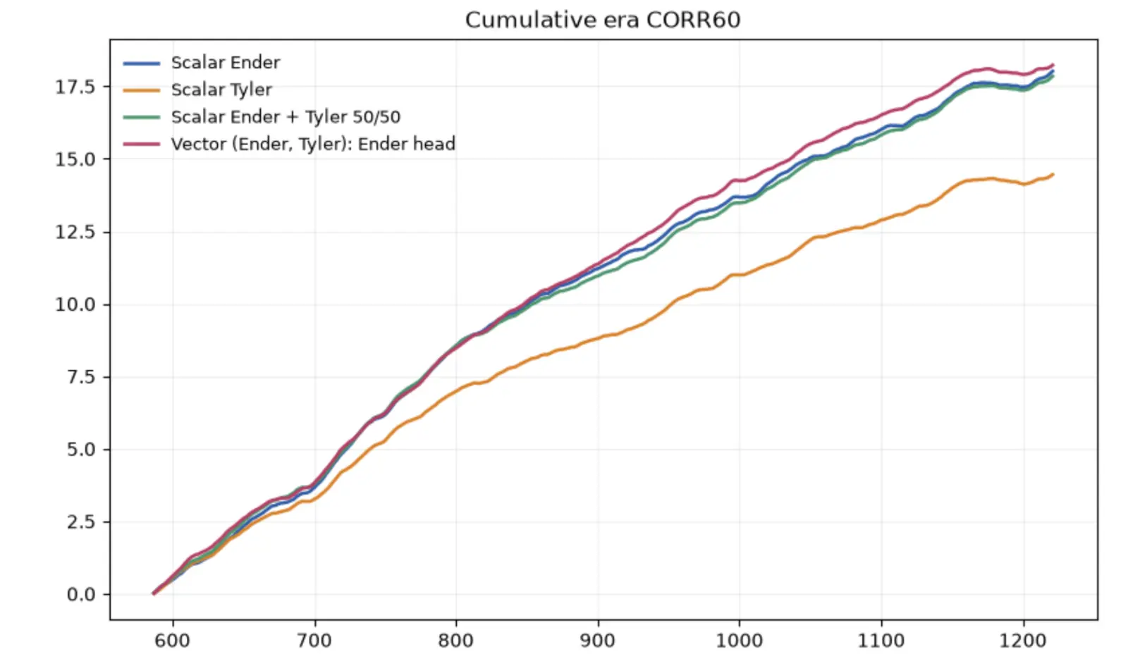
The vector model has the best CORR60 in this experiment. Compared with the scalar Ender model, CORR60 increases from 0.028379 to 0.028705. That is an improvement of 0.000326, or about 1.1% relative. BMC60 changes 0.001126 -> 0.001142.

The difference is small, and this is only one seed and one temporal split. I would treat it as an encouraging signal, not as proof that vector leaves are better for Numerai in general.

Same split budget, better score

I also inspected the saved tree structures to check whether the vector model had simply used more tree capacity.

Candidate	Logical trees	Split nodes	Leaf values	CORR60
Scalar Ender	500	15,500	16,000	0.028379
Vector Ender + Tyler	500	15,500	32,000	0.028705
Scalar pair / 50/50 blend	1,000	31,000	32,000	0.028103

Every tree in all three trained boosters reached depth 5. A complete depth-5 binary tree has 31 split nodes and 32 leaf positions, so each scalar model contains exactly:

500 * 31 = 15,500 split nodes
500 * 32 = 16,000 leaf values

The vector inspection output reports 47,500 counted entries. That does not mean each vector tree has 95 logical node positions. It is 15,500 split nodes plus 32,000 individual leaf values: the same 32 leaf positions per tree, with two target values stored in every leaf.

The complete trees also show that min_child_weight=20 did not prevent any branch from reaching max_depth=5 in either model. This is worth checking, because the parameter could otherwise mean something different in the two settings. XGBoost's documentation states that with vector leaf the mean Hessian across targets is compared against min_child_weight, so the threshold has the same meaning in both models rather than becoming effectively stricter when a second target is added.

This gives the scalar Ender model and the vector model the same split budget. They asked the same number of questions, although not necessarily about the same features or at the same thresholds. The vector model had to choose those splits using both targets and still achieved the best CORR60.

The scalar pair behind the blend used twice as many trees and split nodes. It produced the same total number of leaf values as the vector model, but its final blended prediction scored lower. In this experiment, sharing the tree structure was more effective than combining two independently learned structures after training.

Why the simple blend is interesting

The 50/50 rank average is especially useful to compare with the vector model. Its CORR60 is 0.028103 which is not far from the single Ender model. Its BMC60, however, falls from 0.001126 to -0.000039.

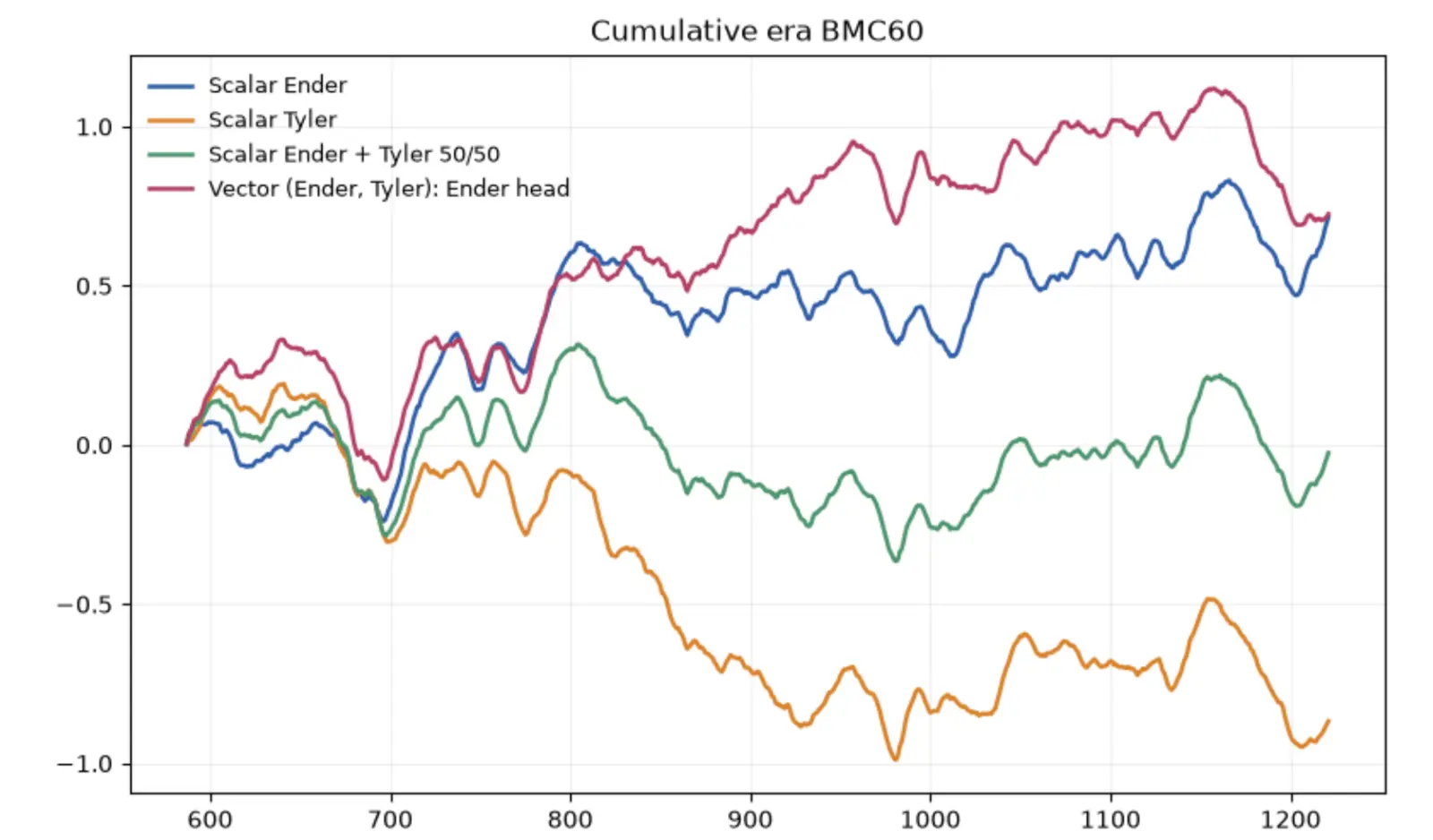
So simply mixing the Tyler prediction into the Ender prediction removed almost all of the benchmark-relative contribution. The vector model does not show the same behavior, even though it is trained using the same two targets. That is an important distinction.

Averaging two predictions happens after both models have already been trained. The tree structures are fixed, and the blend can only interpolate between the two finished predictions. With a vector-leaf model, the targets interact while the trees are being built. Both targets participate in deciding which splits are worth making. The second target therefore influences the representation learned by the model, not just the final prediction.

Training time

With two targets, the vector model did not provide a speed advantage on CPU.

Model	Time
Scalar Ender	2.6 min
Scalar Tyler	2.7 min
Vector Ender + Tyler	5.9 min

Training the two scalar models separately takes about 5.3 minutes in total. The vector model took 5.9 minutes. So for two outputs, there is no training-time win in this experiment. That is not especially surprising. Two targets are the smallest interesting multi-output case. The efficiency argument for vector leaves becomes more relevant as the number of outputs grows, because the default strategy needs another tree for every additional target on every boosting round.

Model size

The shared structure did reduce serialized model size when compared with keeping both scalar models.

Model artifacts	JSON size	UBJ size
Scalar Ender	1.8371 MB	1.3712 MB
Scalar Tyler	1.8374 MB	1.3712 MB
Scalar pair	3.6745 MB	2.7424 MB
Vector Ender + Tyler	2.5259 MB	1.6297 MB

Compared with the scalar pair, the vector model is about 31% smaller in JSON and 41% smaller in UBJ. Both approaches store 32,000 leaf values, but the scalar pair duplicates the tree structure and uses 31,000 split nodes instead of 15,500.

The model-size advantage is therefore real when every output is useful. For a single-output deployment, multi-output training may still improve the score, but storage is not one of its benefits.

When vector leaves make sense

I would consider multi_output_tree when several targets use exactly the same feature rows and there is a reasonable reason to believe they depend on similar parts of the feature space.

This does not require the target values themselves to be highly correlated. What matters is whether the same split questions are useful.

The approach also becomes more attractive as the number of targets grows. With many outputs, creating a separate tree per target on every boosting round increases model size quickly, while a vector tree continues to use one shared structure.

Model size and prediction latency can therefore become practical reasons to try it even before considering any regularization benefit.

I would stay with the default strategy when the targets are genuinely unrelated, when they need different objectives, or when they depend on very different feature structures. Separate trees are more flexible, and sometimes that flexibility is exactly what the problem requires.

A note about boosting rounds

There is one comparison detail that becomes important when the number of targets grows. With the default strategy, every boosting round adds one tree per target. With vector leaves, every boosting round adds one shared tree.

So with 20 targets:

500 scalar rounds = 10,000 trees
500 vector rounds = 500 trees

These models do not have the same amount of structure. The split-node counts earlier in this article show the gap already at two targets, and it widens with every additional output. That means a simple 500-round versus 500-round comparison becomes increasingly unfair as the target count grows. The XGBoost team recommends allowing a generous maximum number of rounds for the vector model, using a lower learning rate, and letting early stopping determine where training should finish. For this experiment, I kept both at 500 rounds because there are only two targets and I wanted the comparison to remain simple. I would not use the same setup for a 20-target experiment.

Limits of this experiment

This test has several obvious limitations. There is one random seed, one temporal split, and one target partner out of 19 possible 60-day targets. The models were not tuned, which keeps the comparison simple but also means neither strategy is necessarily close to its best configuration.

The performance difference is small enough that another seed or another validation window could change the ordering. What the experiment does give us is a clean starting point. The models use the same rows, same features, same parameters, same number of boosting rounds, and the same embargo. The simple scalar blend also provides a baseline for the obvious alternative to multi-output training.

That makes the experiment easy to reproduce and extend. The next steps I would try are several random seeds, walk-forward validation instead of one fixed split, and more than two targets. The higher-output case is especially interesting because that is where the model-size and training-efficiency arguments for vector leaves should become much more visible.

FAQ

What does multi_strategy do in XGBoost?

It controls how XGBoost handles multi-output targets. The default one_output_per_tree creates a separate tree for each target on every boosting round. The alternative, multi_output_tree, creates one shared tree whose leaves contain one prediction value per target.

Is a vector-leaf model always faster?

No. With two targets, my vector model took 5.9 minutes, while the two scalar models took 2.6 and 2.7 minutes. The efficiency advantage becomes more interesting as the number of outputs increases.

Is a vector-leaf model always smaller?

No. It depends on what the deployment would otherwise contain.

In this experiment, the vector model was about 31% smaller in JSON and 41% smaller in UBJ than storing both scalar models. But it was about 37% larger in JSON and 19% larger in UBJ than the Scalar Ender model alone.

If you need every output, shared trees can save substantial space. If you consume only one output, the extra leaf values can make the vector model larger than the single scalar model you would otherwise deploy.

Do the targets need to be strongly correlated?

No. Target correlation and partition compatibility are different ideas. Two weakly correlated targets may still benefit from the same feature splits, while two highly correlated targets may prefer different decision boundaries. In this experiment, the partner target was deliberately chosen from the least correlated targets in the 60-day family.

Can I just train two models and average them?

Yes, and I think that is an important baseline to test.

In this experiment, however, the 50/50 rank average performed differently from the vector model. It retained much of the raw CORR but lost almost all of the BMC contribution. It also used 31,000 split nodes across two scalar models, compared with 15,500 in the vector model, and still achieved lower CORR60. The reason is structural. Averaging combines predictions after training. A vector model allows both targets to influence the tree splits during training.

Which XGBoost version should I use?

The multi_strategy parameter appeared in XGBoost 2.0, but the implementation was incomplete for several releases. I would use 3.4 or later, which is where the hist implementation became feature-complete. I ran this experiment on 3.4.1.

Does it work on GPU?

Yes. In XGBoost 3.4.1 the hist vector-leaf implementation supports CPU and CUDA training, along with categorical splits and reduced-gradient training.

Further reading

The XGBoost multi-output tutorial covers the official API and current limitations.

The XGBoost team also published Introducing the XGBoost Vector-Leaf Model, with their own experiments on multiclass data.

If you want to inspect tree structures visually, supertree can help with that.

And if you would rather automate model selection and tuning, mljar-supervised provides an AutoML layer around common tabular machine-learning workflows.

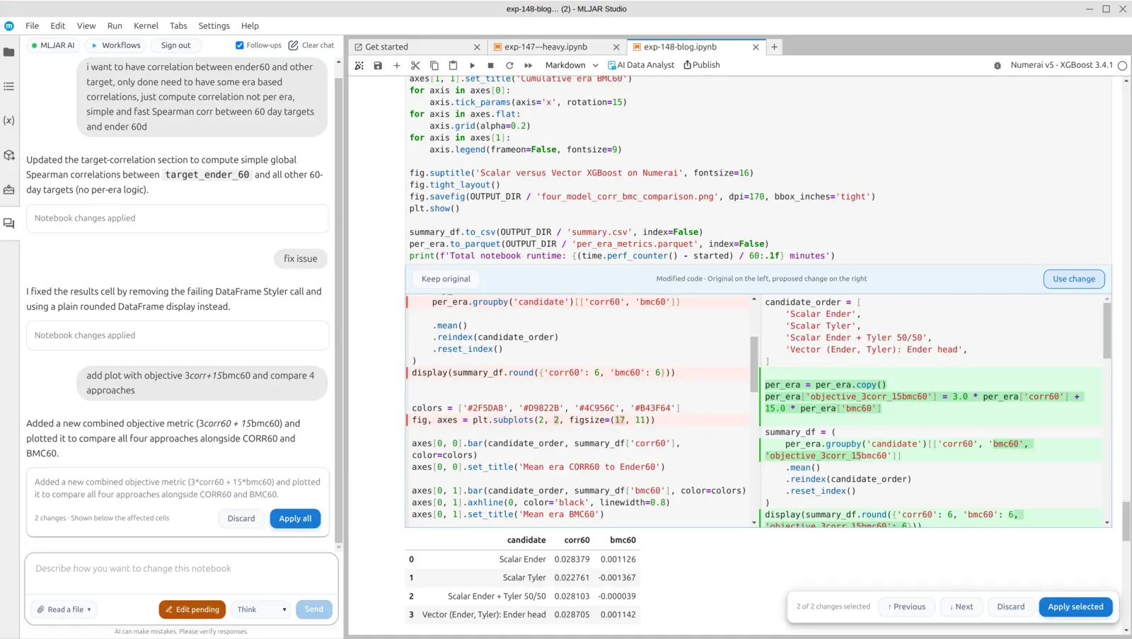
Computing the experiment in MLJAR Studio

I used MLJAR Studio to prepare the notebook, run the computations, inspect the results, and iterate on the analysis with its AI Data Analyst.