In this tutorial, we will use machine learning to predict employee attrition. Employee attrition means that an employee leaves the company. It is an important topic for HR teams because losing good employees can be expensive and difficult for the company. People leave jobs for many reasons. Sometimes it is because of salary. Sometimes it is because of overtime, low job satisfaction, long distance from home, work-life balance, or limited career growth. Every person has a different story, but data can help us find common patterns.
If a company can find employees who may be at risk of leaving, it can react earlier. For example, the company can talk with the employee and ask what can be improved in the workplace. Sometimes a better career path, a bonus, a salary raise, more flexible work, or a simple honest conversation can help keep a good employee. This can be a win-win situation. The employee can get better working conditions, and the company can keep a qualified person. It can also save time and money, because hiring and training a new employee is often expensive.
We will use AutoML to make the machine learning workflow easier. AutoML will train several models for us, compare their performance, and prepare useful reports. We will also check if the best model is fair for the Gender feature. This tutorial is beginner friendly. You do not need to know advanced machine learning. We will go step by step. All code in this tutorial was prepared in MLJAR Studio, a desktop application for data science. MLJAR Studio installs Python and prepares the working environment for you. You can focus on learning and working with data instead of spending time on technical setup.
Of course, machine learning should not be used to make automatic HR decisions. It should be used as a support tool. The model can help HR teams find useful signals in the data, but the final decision should always include human understanding and respect for the employee.
What You Will Learn
In this tutorial, you will learn how to:
- load HR data with Python,
- understand what one row in a DataFrame describes,
- define features and target,
- prepare a simple machine learning task,
- use AutoML to train and compare models,
- inspect the model leaderboard,
- check feature importance,
- review model performance,
- understand fairness metrics for Gender,
- use machine learning in HR in a responsible way.
Data
We will use an employee attrition dataset. The dataset contains information about employees and whether they left the company. Let's load the data with Python.
import pandas as pd from IPython.display import display url = "https://raw.githubusercontent.com/pplonski/datasets-for-start/master/employee_attrition/HR-Employee-Attrition-train.csv" df = pd.read_csv(url) df.head()
This code loads the data from a CSV file and displays the first rows of the dataset.
The dataset has 1200 rows and 35 columns. Here is an example view of the data:
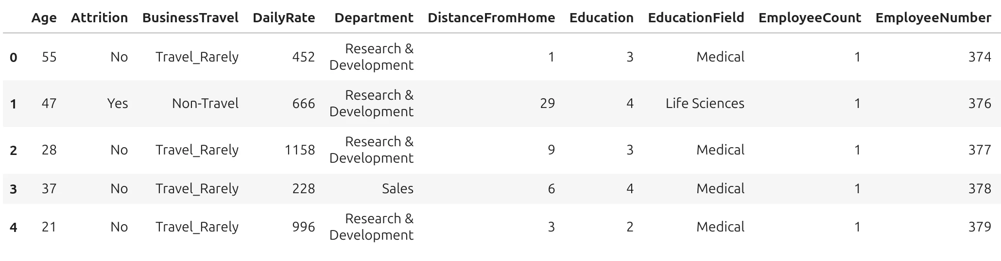
Each row is one employee. Each column describes one property of this employee.
The dataset contains columns such as:
Age,BusinessTravel,Department,DistanceFromHome,EducationField,EnvironmentSatisfaction,Gender,JobLevel,JobSatisfaction,MonthlyIncome,OverTime,TotalWorkingYears,WorkLifeBalance,YearsAtCompany,Attrition.
The most important column for us is Attrition. This is the column that we want to predict.
What Does One Row Describe?
One row in the data table describes one employee.
For example, the first row has index 0. It describes an employee who is 55 years old, did not leave the company, travels rarely, works in Research & Development, and lives 1 unit of distance from work. This employee has many years of work experience and many years at the company.
This row is like a small employee profile. It does not tell us everything about the person, but it gives us useful information for analysis. The model looks at many rows like this and tries to learn patterns. For example, it can learn that overtime, job satisfaction, job level, age, or distance from home can be connected with employee attrition.
Features and Target
In machine learning, we often use two important words:
- features - columns used to make predictions,
- target - column we want to predict.
In this dataset, the target is Attrition.
The Attrition column tells us if an employee left the company or stayed. It has two possible values:
Yes - the employee left the company No - the employee stayed in the company
This is a classification task because the model predicts one of two classes. We will use other columns as features. These features describe the employee and the job situation. The model will learn from these features and try to predict the target.
Prepare Features, Target, and Sensitive Feature
In this tutorial, we also want to check model fairness for the Gender feature.
We will use Gender as a sensitive feature for fairness analysis. It means that we want to check if the model behaves similarly for different gender groups. We will not use Gender directly as an input feature for prediction. We remove it from X, but we keep it separately for fairness checks.
import pandas as pd from supervised import AutoML y = df["Attrition"].copy() sensitive = df[["Gender"]].copy() # Exclude target, ID-like column, and sensitive feature from predictors X = df.drop(columns=["Attrition", "EmployeeNumber", "Gender"])
Let's explain this code. The variable y contains the target. This is the real attrition value. The variable sensitive contains the Gender column. We will use it later to check fairness. The variable X contains input features. We remove:
Attrition, because this is the target,EmployeeNumber, because it is an ID-like column,Gender, because we do not want to use it directly for prediction.
This is an important step. We want to build a model that predicts attrition and then check if the predictions are fair for different gender groups.
Basic Machine Learning Pipeline
A basic machine learning pipeline has several steps. First, we load the data. Then we select the target column. Next, we prepare input features. After that, we train a machine learning model and evaluate it on data that was not used during training.
In a manual workflow, we would need to select an algorithm, prepare preprocessing, tune parameters, train the model, compare results, and inspect the final model. This can take time. It can also be difficult for beginners because there are many algorithms and many settings. This is why we will use AutoML.
What Is AutoML?
AutoML means Automated Machine Learning. AutoML helps automate many repetitive steps in a machine learning project. It can train different algorithms, compare their performance, and prepare reports with metrics and charts. In this tutorial, AutoML will train several models for employee attrition prediction. It will check models such as: Baseline, Linear model, Decision Tree, Random Forest, XGBoost, Neural Network, Ensemble. AutoML does not mean that we can stop thinking. We still need to understand the data, inspect the results, and decide if the model makes sense. But AutoML helps us move faster. Instead of manually testing many algorithms, we can let AutoML do this work and then focus on interpretation.
Run AutoML
Now we can run AutoML.
automl = AutoML( mode="Explain", results_path="automl_attrition_explain_gender", eval_metric="auc", random_state=42 ) automl.fit(X, y, sensitive_features=sensitive)
Let's explain the most important parameters. The parameter mode="Explain" tells AutoML to train models and prepare explanations. The parameter eval_metric="auc" tells AutoML to optimize the AUC metric. AUC is a popular metric for binary classification. It helps measure how well the model separates two classes. The parameter random_state=42 makes the results easier to reproduce.
The method:
automl.fit(X, y, sensitive_features=sensitive)
means:
Train models using input features
X, targety, and useGenderfor fairness analysis.
During training, AutoML prints information about the process.
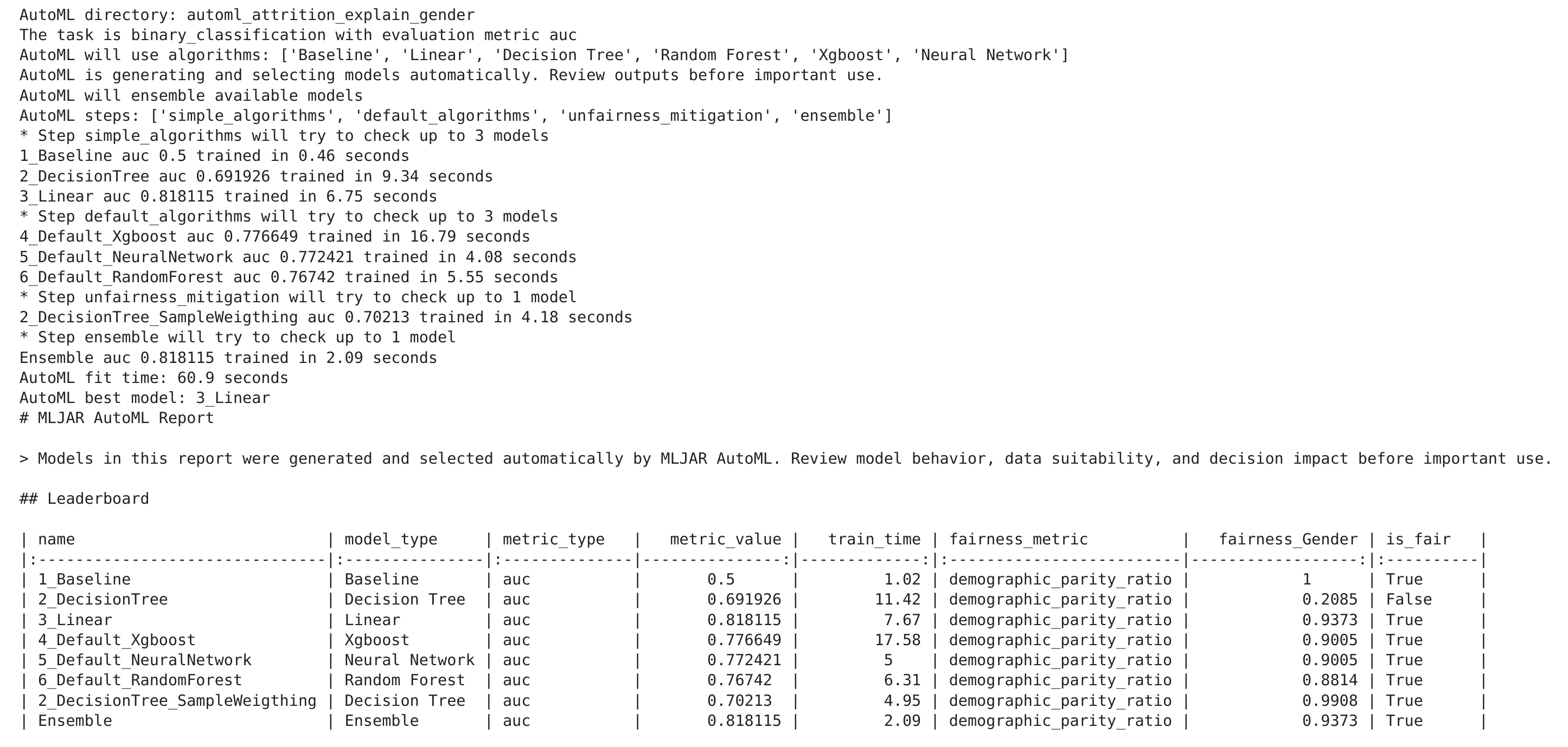
AutoML trained several models automatically. It also created a report with performance metrics, feature importance, and fairness information.
AutoML Report
After training, we can display the AutoML report.
automl.report()
The report is useful because it gives us many important results in one place. We can inspect trained models, compare metrics, check feature importance, and review fairness.
In HR, this is very important. We do not want to look only at model performance. We also want to check if the model behaves fairly for different groups. A model can have good accuracy and still be problematic. That is why fairness analysis is part of this tutorial.
Model Leaderboard
The AutoML leaderboard shows all trained models and their scores.
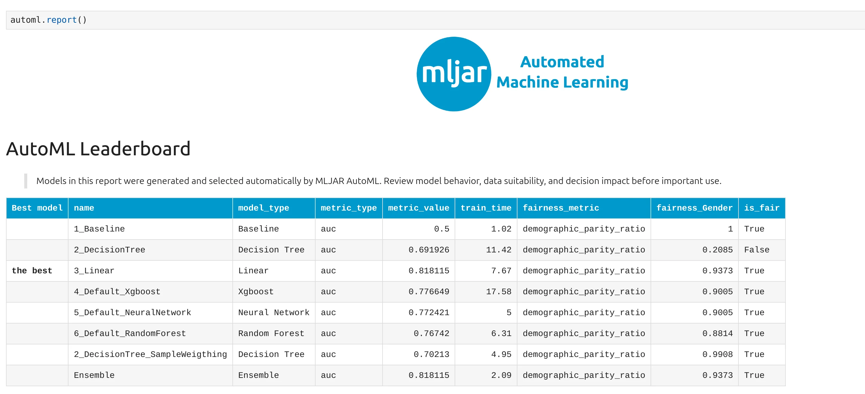
The leaderboard helps us quickly compare models. We can see model names, model types, metric values, training time, fairness metric, and fairness status. In this experiment, the best model is 3_Linear. It achieved an AUC score of about 0.818115. This is a nice result. The Linear model performed well and passed the fairness check for Gender.
There is also an Ensemble model with the same AUC score. However, the best selected model is the Linear model because Enseble was constructed only from one model, guess which one? This is great for a beginner tutorial because linear models are usually easier to understand than more complex models.
AutoML Performance Plot
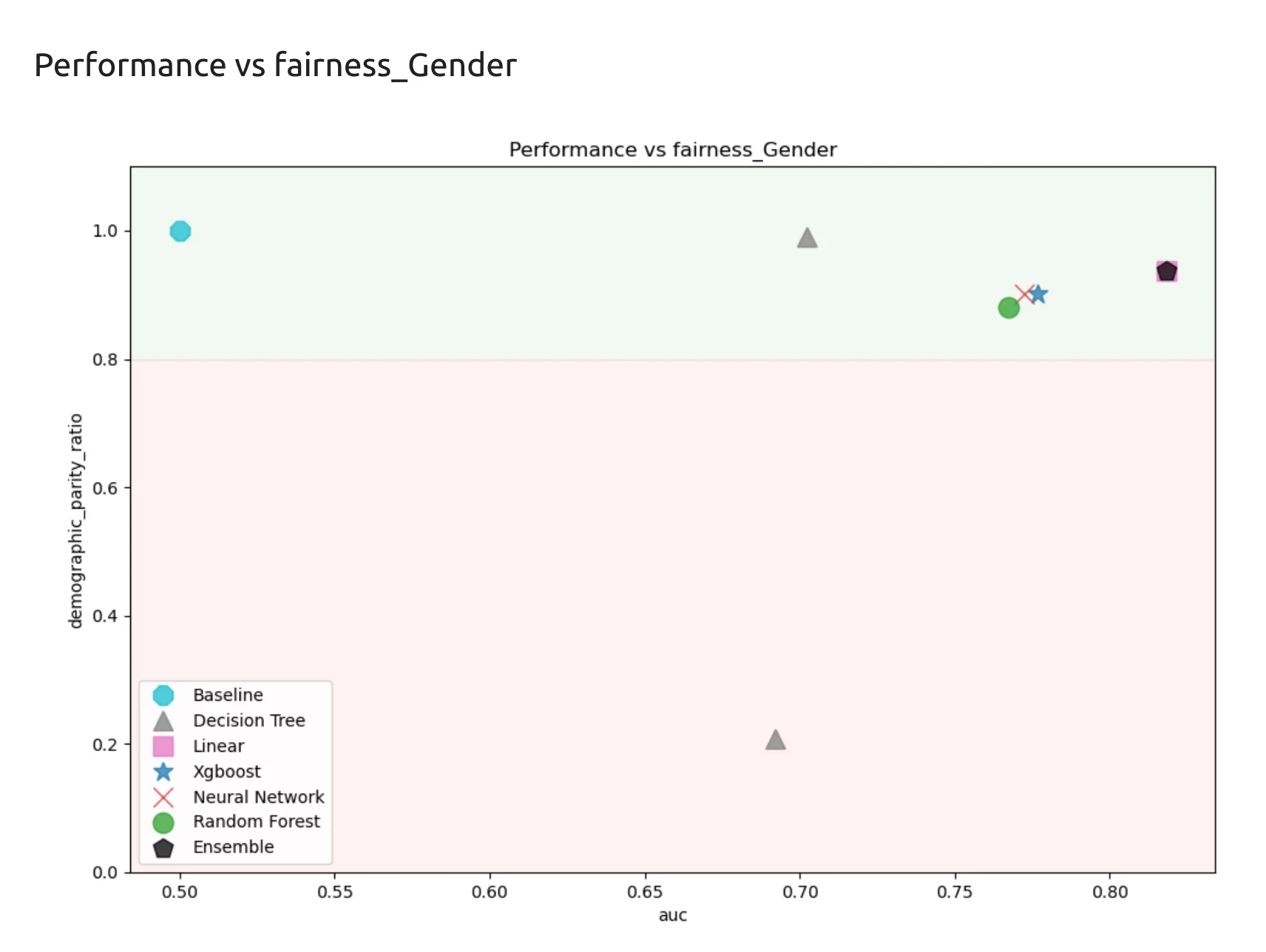
A table is useful, but a chart can make model comparison easier.
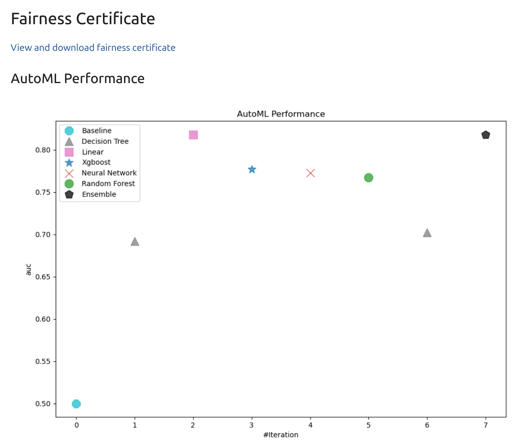
The performance plot helps us see how different models compare. We can quickly check which models performed better and which models were weaker. In this experiment, the Linear model is at the top. It gives a strong result and is easier to explain than many black-box models.
Why the Linear Model Is Useful
Linear models are often a good starting point for tabular data. They are not always the most powerful models, but they are usually easier to understand. This is especially important in HR. If we build a model that can affect people, we should be able to explain how it works.
In this tutorial, the best model is not only accurate. It is also easier to inspect. This is a good combination:
Good performance plus better explainability.
Linear Model Performance Metrics
Let's inspect the performance metrics for the best Linear model.
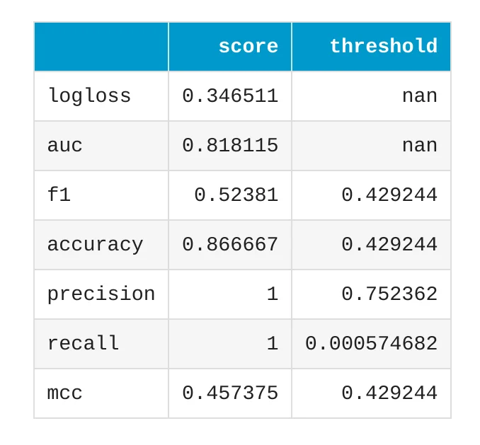
The model has accuracy around 0.8667 on the validation data. Accuracy tells us how often the model predicted the correct class. For example, if accuracy is 0.8667, it means that the model was correct in about 86.67% of validation examples.
However, accuracy is not the only metric we should check. In attrition prediction, the positive class is usually smaller than the negative class. Many employees stay, and fewer employees leave. In such cases, we should also inspect metrics like AUC, true positive rate, false negative rate, and false positive rate. Good metrics do not mean that the model is ready for automatic HR decisions. Metrics help us understand the model, but they are only one part of responsible machine learning.
ROC Curve
The ROC curve is another way to inspect a binary classification model.
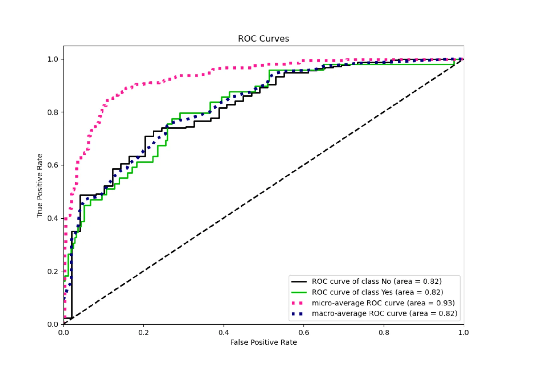
The ROC curve shows how well the model separates two classes:
Attrition = Yes Attrition = No
It is enough to remember this:
A better ROC curve means that the model is better at separating employees who left from employees who stayed.
We do not need to go deep into the formula here. The most important idea is that ROC helps us look at model quality from a different angle than accuracy.
Feature Importance Across Models
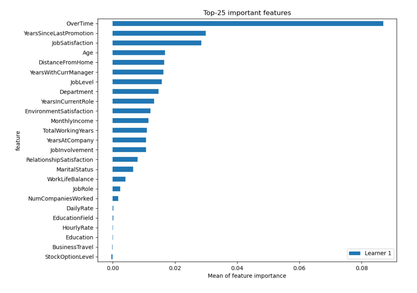
After training models, we want to know which features were useful for prediction. AutoML can show global feature importance averaged across models.
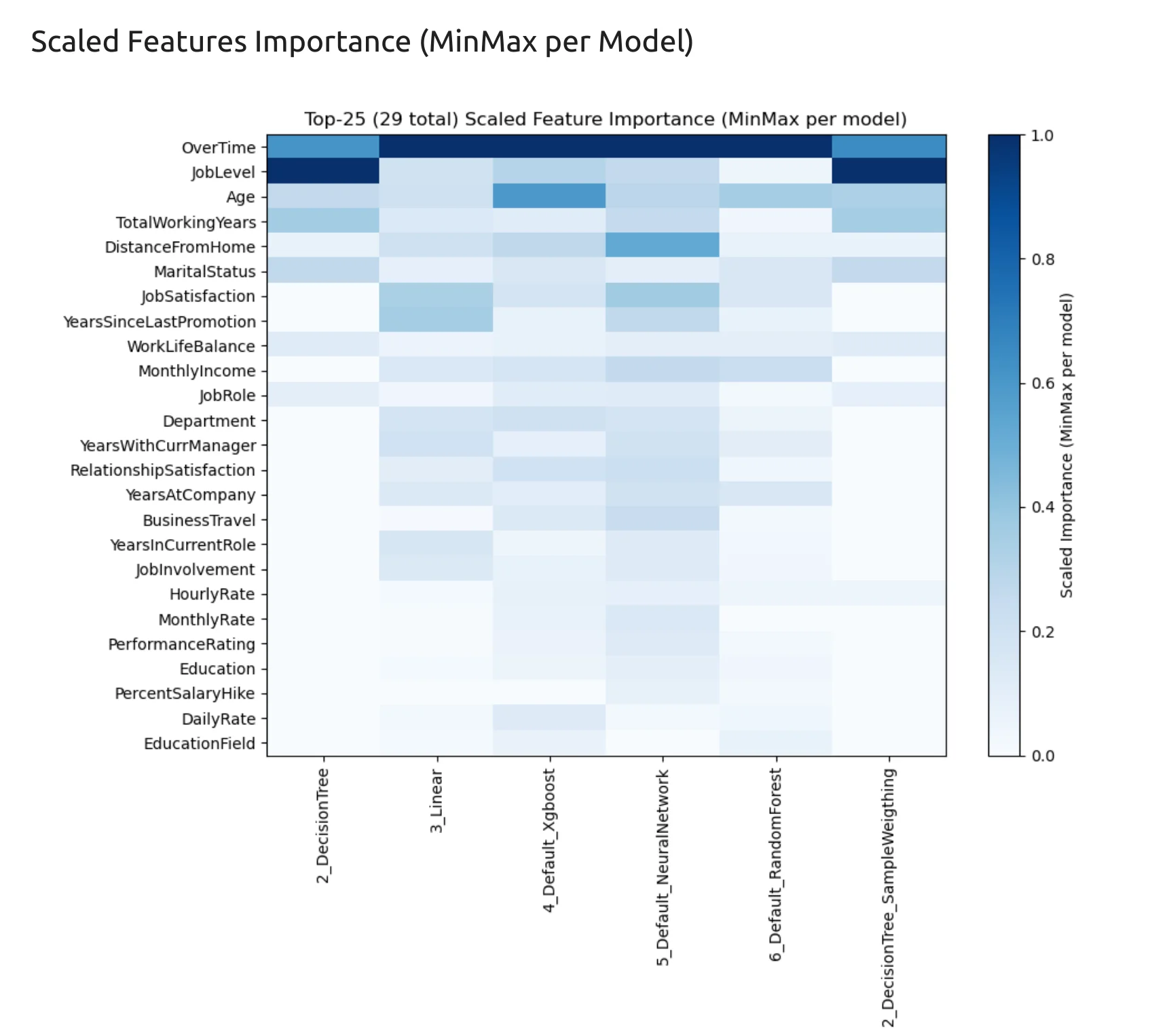
The most influential features in this experiment include:
OverTime,Age,JobLevel,DistanceFromHome,JobSatisfaction,TotalWorkingYears,MaritalStatus,MonthlyIncome,Department,WorkLifeBalance.
These features make sense in an HR attrition problem. Overtime, job satisfaction, job level, income, and work-life balance can all be connected with the decision to leave a company. But we need to be careful with interpretation. Feature importance does not prove causation. It does not mean that one feature directly causes attrition. It only means that the model found this feature useful for prediction in this dataset.
Feature Importance for the Linear Model
We can also inspect feature importance for the best Linear model.
This chart helps us understand which features had the strongest influence in the selected model. Feature importance is useful because it makes the model less mysterious. Instead of only getting predictions, we can also ask:
- Which columns mattered most?
- Do these columns make sense?
- Are there any surprising features?
- Should we inspect the data more carefully?
This is very important in HR analytics. We should not blindly trust a model. We should inspect what it learned.
Linear Model Coefficients
Linear models can also be inspected with coefficients.
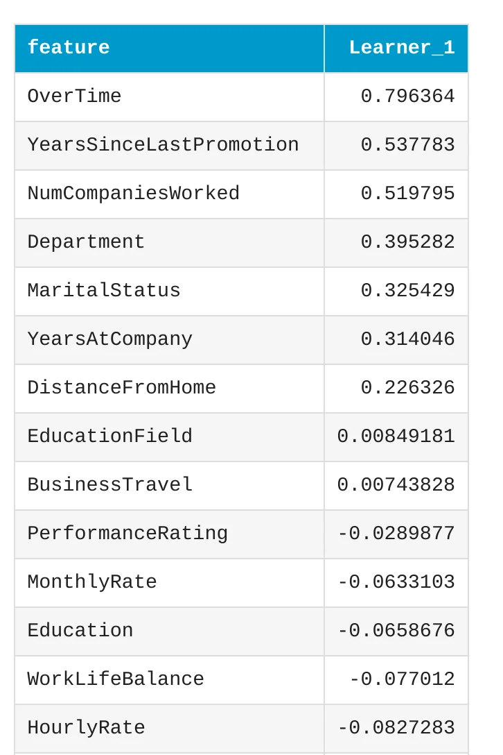
A coefficient tells us how a feature is connected with the model prediction. Some coefficients can push the prediction toward attrition (large positive coefficient value). Other coefficients can push the prediction toward staying in the company (negative coefficients). This is one reason why linear models are useful. They are easier to explain than many complex models. We can look inside and understand what features are important. Still, coefficients should be interpreted carefully. Real HR problems are complex. A model can show useful patterns, but it does not understand the full human context.
SHAP Explanations for Good Decisions
AutoML also gives SHAP explanations. SHAP is a method that helps explain individual predictions. It can show which features pushed a prediction in one direction or another.
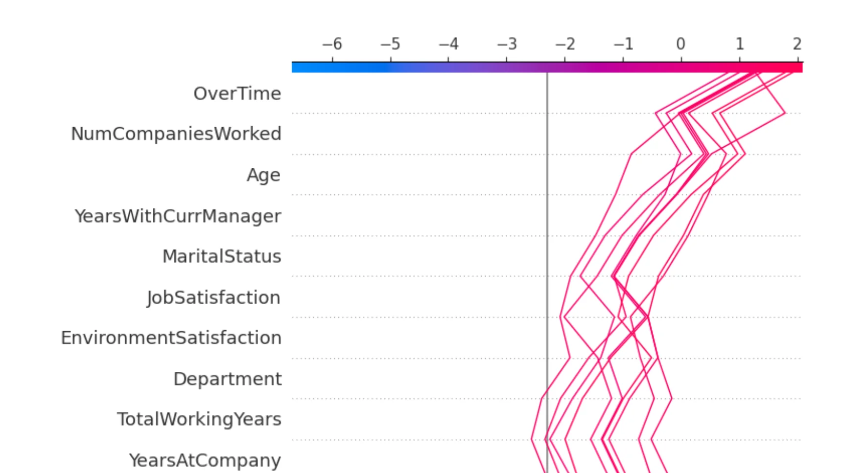
This chart shows examples where the model made good decisions for class 1. In this tutorial, class 1 means attrition. This is useful because we can see which features helped the model correctly detect employees who left the company.
SHAP Explanations for Wrong Decisions
It is also important to inspect mistakes.
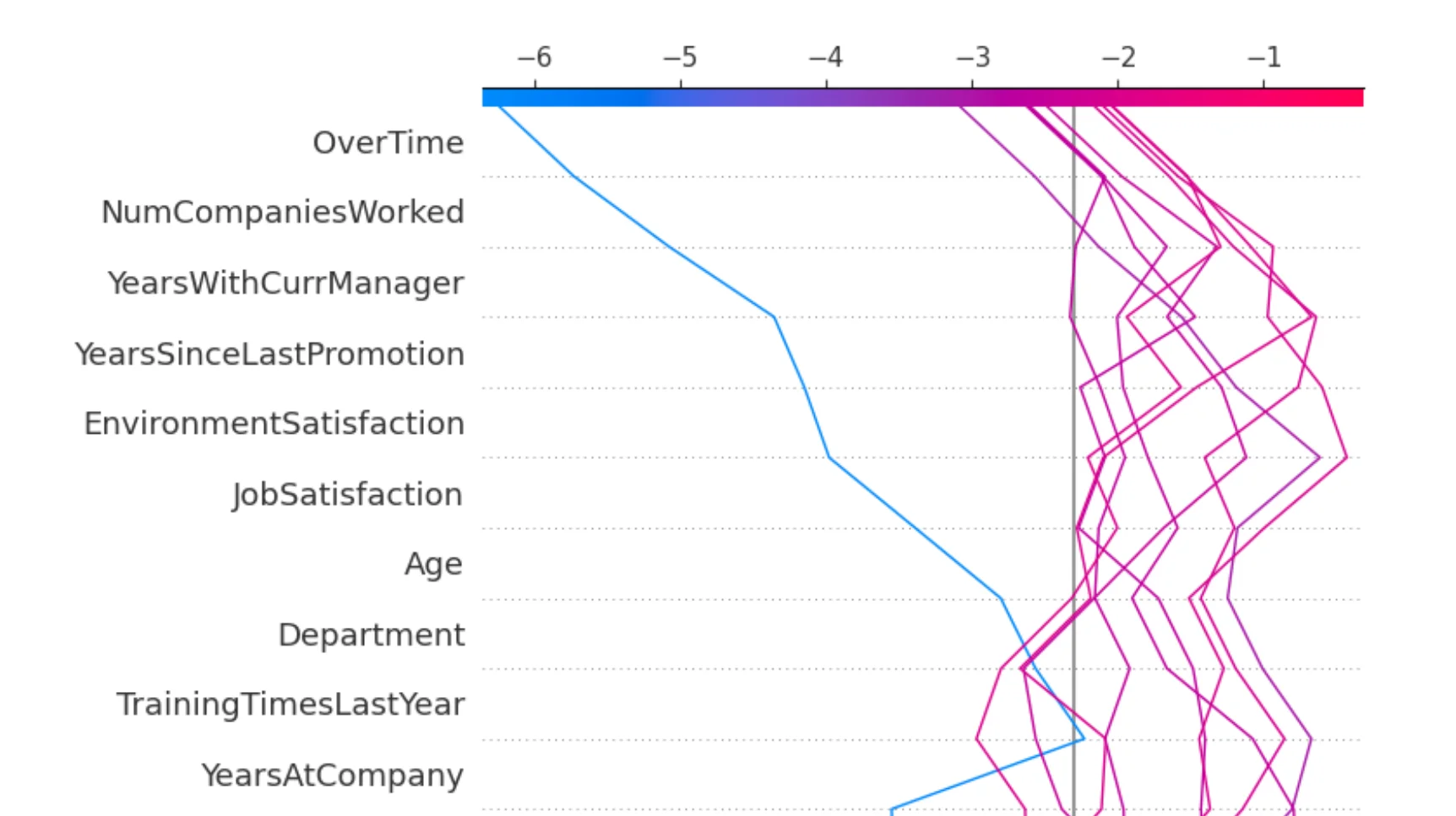
This chart shows examples where the model made worse decisions for class 1. This is very useful in real machine learning work. We should not look only at successful predictions. We should also inspect errors and ask why they happened. A model can work well on average and still fail on some important cases. Error analysis helps us understand these situations.
Why Fairness Matters in HR
HR is a sensitive area. Machine learning models used with HR data must be handled carefully. A model can have good performance and still behave differently for different groups. For example, it could make more mistakes for one group than another. It could select one group more often. It could have different false positive or false negative rates.
This is why fairness analysis is important. In this tutorial, we check fairness for the Gender feature. We removed Gender from the input features, so the model does not use it directly for prediction. But we still use Gender as a sensitive feature to check model behavior after training.
This helps us answer an important question:
Does the model behave similarly for Male and Female employees?
Fairness Certificate
MLJAR AutoML can prepare a fairness certificate for the trained model.
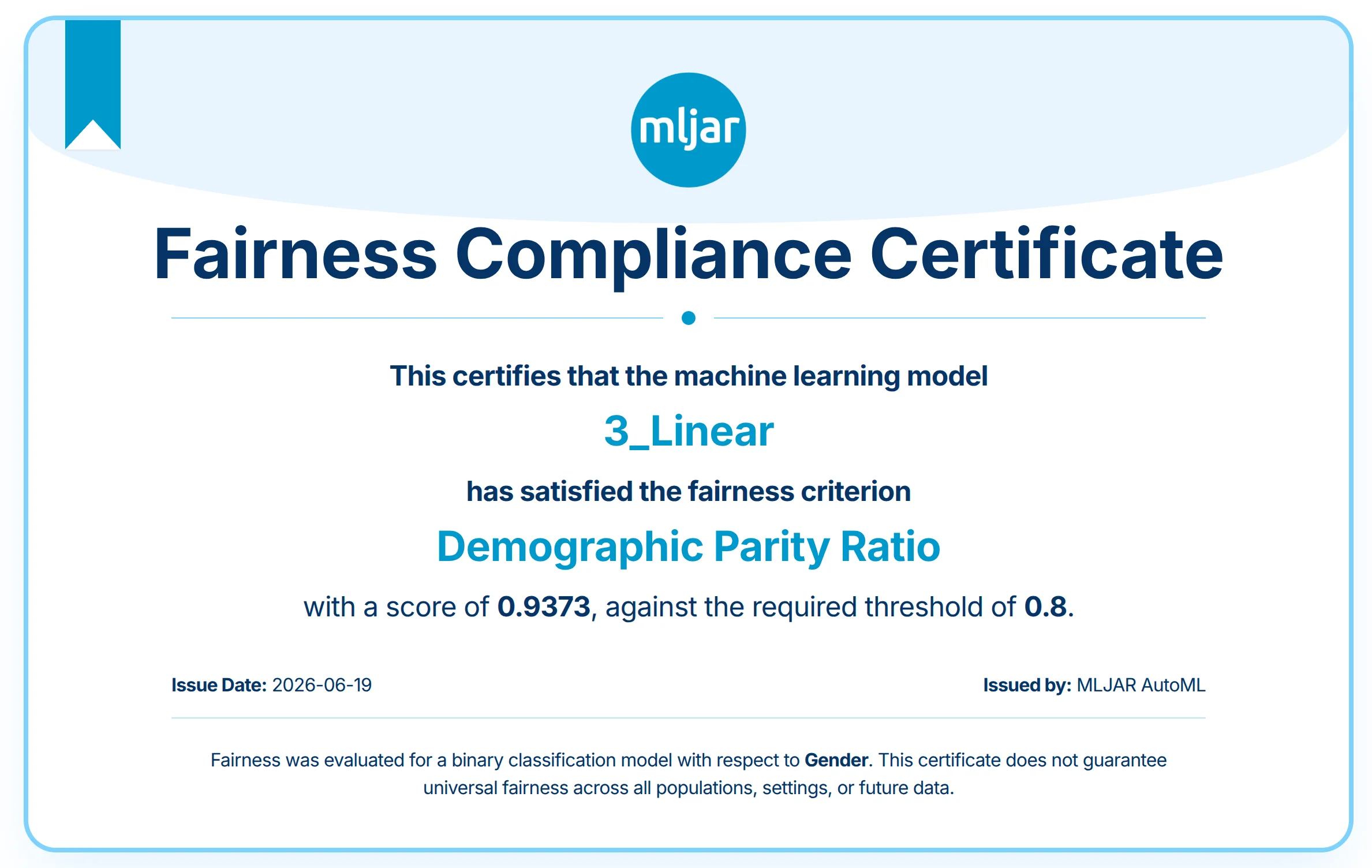
The fairness certificate gives a quick summary of the fairness check.
You can see the fairness certificate in MLJAR website - it is generated automatically.
In this experiment, the fairness metric is:
Demographic Parity Ratio
The required threshold is:
0.8
The achieved score for the best model is:
0.9373
The model passed this fairness check for the Gender feature.
This is a good sign, but we should still inspect the detailed metrics. A certificate is useful as a summary, but responsible machine learning needs more than one number.
Selection Rate for Gender
Selection rate tells us how often the model predicts the positive class for each group. In our case, the positive class is attrition. So selection rate tells us how often the model predicts that an employee may leave.
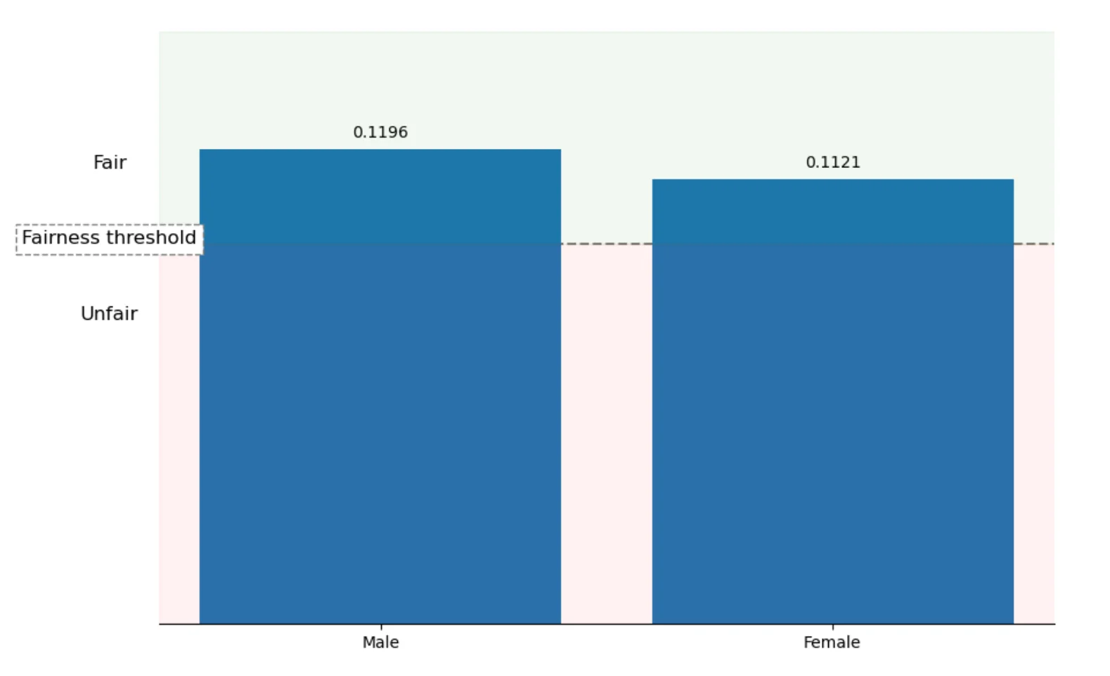
For the Linear model, the selection rates are:
| Group | Selection Rate |
|---|---|
| Male | 0.1196 |
| Female | 0.1121 |
These values are very close. The difference is 0.0075. This means that the model predicts attrition at a similar rate for Male and Female employees. This is a good fairness signal.
False Rates for Gender
Selection rate is useful, but it is not enough. We should also inspect error rates.
A false positive means:
The model predicts attrition, but the employee actually stays.
A false negative means:
The model predicts staying, but the employee actually leaves.
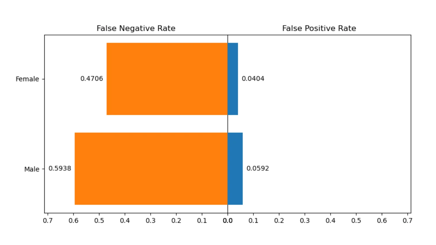
False positives and false negatives are important because they tell us what kind of mistakes the model makes. In HR attrition prediction, a false negative can mean that the model misses an employee who is at risk of leaving. A false positive can mean that the model marks an employee as at risk, even though the employee stays. Both types of mistakes matter. That is why we inspect them separately.
Fairness Metrics for Gender
Now let's look at the detailed fairness metrics for the Linear model.
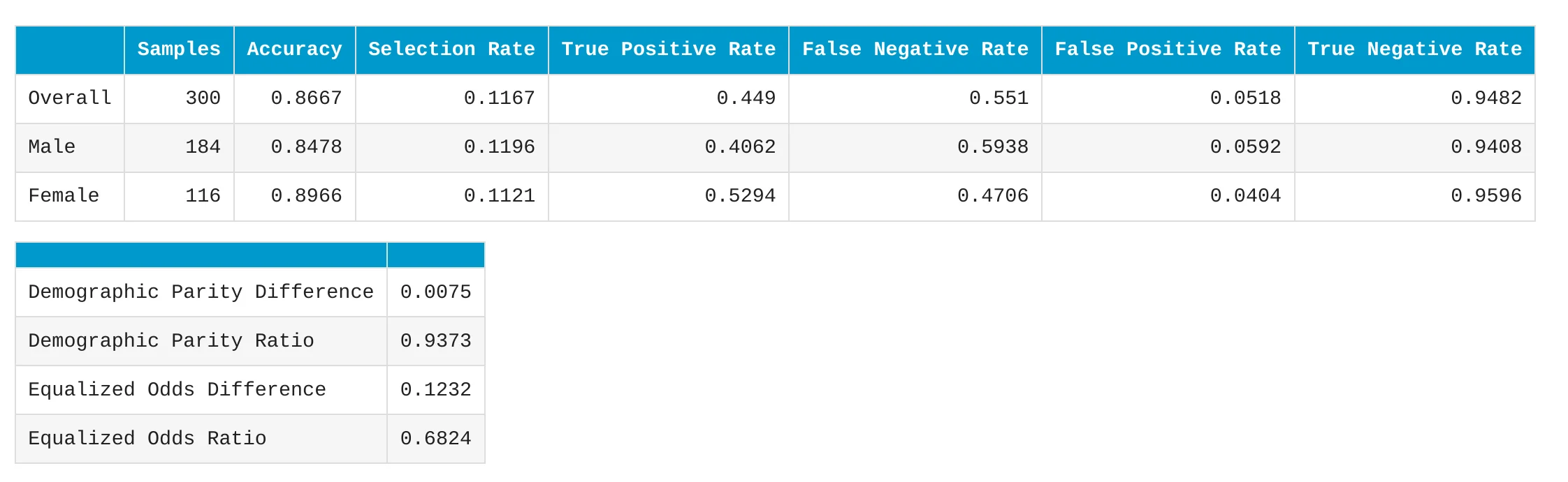
The table shows that the model has similar selection rates for Male and Female employees. The accuracy is also good for both groups.
There are some differences in true positive rate and false negative rate. For example, the true positive rate is higher for Female employees than for Male employees. This means the model detected a higher share of real attrition cases in the Female group. This is why it is useful to look at more than one fairness metric. A model can look good in one metric and still need more inspection in another metric.
The Demographic Parity Difference is very small. It means that the difference in selection rates between Male and Female groups is small. The Demographic Parity Ratio is 0.9373. This is close to 1, which means that the selection rates are similar. It also passes the fairness threshold of 0.8. The Equalized Odds metrics look at differences in error behavior between groups. These metrics help us check if the model makes similar types of mistakes for different groups.
Fairness is not only one number. It is better to inspect several metrics and understand the business context.
Responsible Use of Machine Learning in HR
Machine learning can be useful in HR analytics, but it should be used carefully. A model can help HR teams find patterns in data. It can support retention analysis. It can help identify which factors are connected with attrition. It can also help managers understand where employee experience may need improvement.
But the model should not make automatic HR decisions. It should not automatically decide who should be promoted, fired, hired, or contacted. HR decisions affect real people, so they need human review, company policy, legal requirements, and ethical thinking.
Machine learning should be a support tool, not a replacement for human judgment.
Why This Is Useful in HR
HR data is often tabular. It can include employee age, department, salary, satisfaction scores, travel frequency, overtime, work-life balance, and years at the company. This kind of data is a good fit for machine learning. A model can find patterns that are difficult to see manually.
AutoML makes this process easier because it can train many models and prepare reports automatically. This is useful for HR analysts, data analysts, and beginner data scientists who want to move faster. The fairness report is also important. It helps us check if the model behaves similarly for sensitive groups. In this tutorial, we checked Gender, but in other projects you may need to check other sensitive features, depending on the data and the use case.
Summary
In this tutorial, we walked through an AutoML workflow for HR analytics. We started with an employee attrition dataset. We explained that each row describes one employee and each column describes one property of this employee. Then we selected Attrition as the target column and prepared input features for machine learning.
We used MLJAR AutoML to train and compare several models. The best model was the Linear model. It achieved strong performance and passed the fairness check for Gender. We inspected the model leaderboard, performance plots, feature importance, model coefficients, SHAP explanations, and fairness metrics.
The most important lesson is simple:
AutoML helps us move faster, and fairness reports help us build more responsible machine learning systems.
Machine learning in HR should always be used with care. Good predictions are useful, but explainability and fairness are just as important.