How to use early stopping in Xgboost training?
Quick answer: Early stopping in XGBoost helps prevent overfitting by selecting the best iteration based on validation performance.
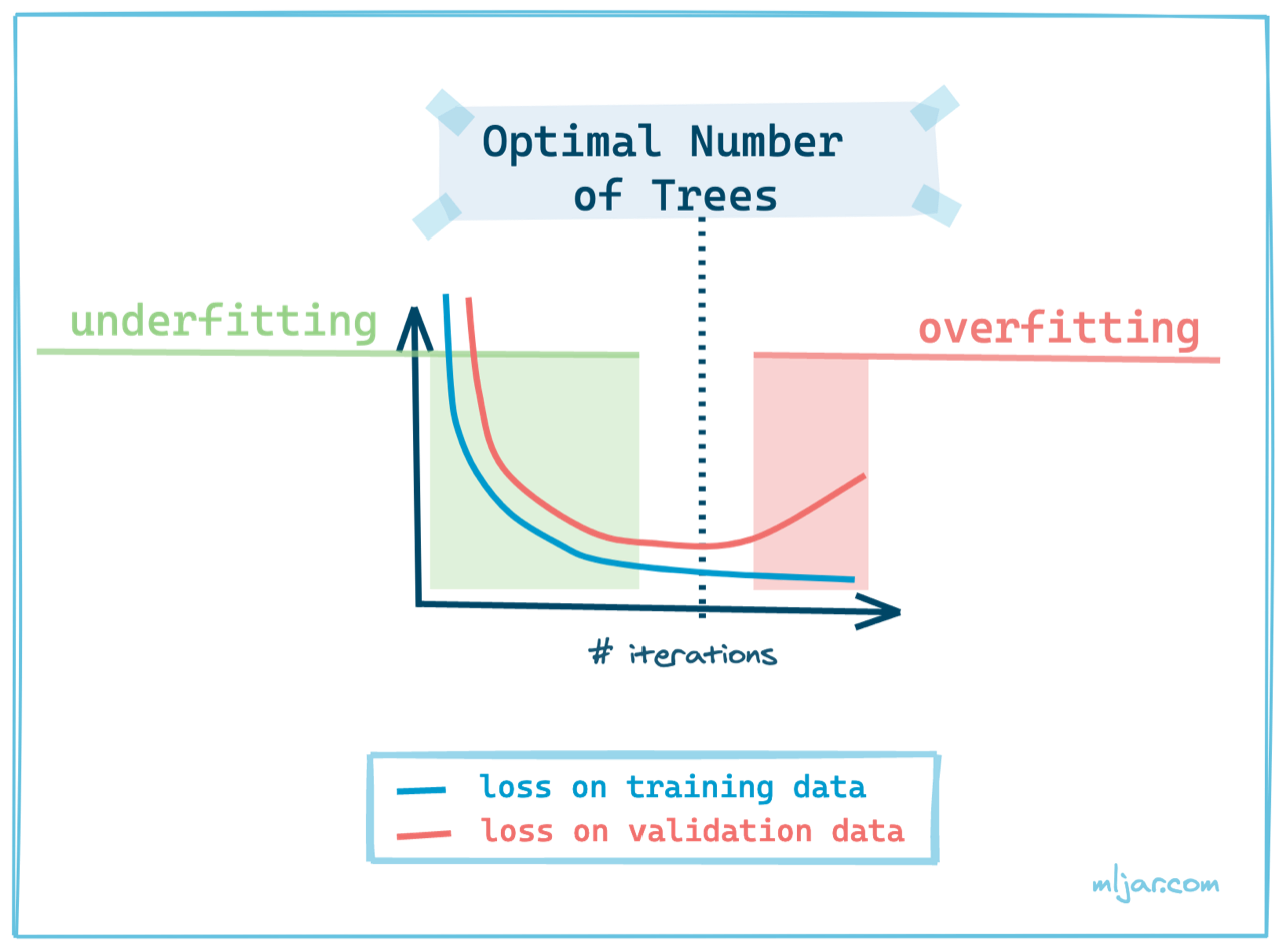
 Xgboost is a powerful gradient boosting framework that can be used to train Machine Learning models. It is important to select optimal number of trees in the model during the training. Too small number of trees will result in underfitting. On the other hand, too large number of trees will result in overfitting. How to find the optimal number of trees? You can use an early stopping. We are using Xgboost in version `2.0.0` in this article. Please update `xgboost` package if you have older version.
Early Stopping
Early stopping is a technique used to stop training when the loss on validation dataset starts increase (in the case of minimizing the loss). That's why to train a model (any model, not only Xgboost) you need two separate datasets:
- training data for model fitting,
- validation data for loss monitoring and early stopping.
In the Xgboost algorithm, there is an early_stopping_rounds parameter for controlling the patience of how many iterations we will wait for the next decrease in the loss value. We need this parameter because the loss values decrease randomly in each iteration. The validation loss can bounce in some range and after few iterations decrease.
How many iterations should early stopping take? I'm using 50 rounds for early stopping (usually with 1000 trees). There are some heuristics that recommend to use 10% of your total iterations for early stopping, which sounds reasonable.
Implementation
Let's show some code example, how to use early stopping during Xgboost training. I'll be using Xgboost API that is Scikit-Learn compatible, because Learning API of Xgboost requires manual handling of best_iteration for prediction and saving (check this article for details).
Create example data
We will create synthetic data set with sklearn package and split it to tain and validation samples.
# load needed packages
import xgboost as xgb
from sklearn.datasets import make_classification
from sklearn.model_selection import train_test_split
from matplotlib import pyplot as plt

# create dataset
X, y = make_classification(n_samples=100,
                           n_informative=5,
                           n_classes=2)
X_train, X_validation, y_train, y_validation = train_test_split(X,
                                                              y,
                                                              test_size=0.25)
Train Xgboost with Early Stopping
Let's train the Xgboost model. I set the hyparameters values max_depth=6, abd learning_rate=0.1 to quickly show the overfitting. The early_stopping_rounds=20 is set for example purposes.
model = xgb.XGBRegressor(n_estimators=100, max_depth=6,
                         learning_rate=0.1, early_stopping_rounds=20)
model.fit(X_train, y_train,
            eval_set=[(X_train, y_train), (X_validation, y_validation)])
The output from model training:
> [0]	validation_0-rmse:0.45517	validation_1-rmse:0.47108
[1]	validation_0-rmse:0.41445	validation_1-rmse:0.44976
[2]	validation_0-rmse:0.37746	validation_1-rmse:0.43300
[3]	validation_0-rmse:0.34385	validation_1-rmse:0.41747
[4]	validation_0-rmse:0.31332	validation_1-rmse:0.40777
[5]	validation_0-rmse:0.28611	validation_1-rmse:0.39987
[6]	validation_0-rmse:0.26140	validation_1-rmse:0.39421
[7]	validation_0-rmse:0.23905	validation_1-rmse:0.39036
[8]	validation_0-rmse:0.21876	validation_1-rmse:0.38798
[9]	validation_0-rmse:0.19948	validation_1-rmse:0.38513
[10]	validation_0-rmse:0.18195	validation_1-rmse:0.38333
[11]	validation_0-rmse:0.16601	validation_1-rmse:0.38237
[12]	validation_0-rmse:0.15152	validation_1-rmse:0.38204
[13]	validation_0-rmse:0.13834	validation_1-rmse:0.38220
[14]	validation_0-rmse:0.12636	validation_1-rmse:0.38271
[15]	validation_0-rmse:0.11546	validation_1-rmse:0.38348
[16]	validation_0-rmse:0.10567	validation_1-rmse:0.38314
[17]	validation_0-rmse:0.09681	validation_1-rmse:0.38311
[18]	validation_0-rmse:0.08878	validation_1-rmse:0.38331
[19]	validation_0-rmse:0.08159	validation_1-rmse:0.38168
[20]	validation_0-rmse:0.07498	validation_1-rmse:0.38157
[21]	validation_0-rmse:0.06904	validation_1-rmse:0.37995
[22]	validation_0-rmse:0.06361	validation_1-rmse:0.38003
[23]	validation_0-rmse:0.05847	validation_1-rmse:0.38143
[24]	validation_0-rmse:0.05380	validation_1-rmse:0.38274
[25]	validation_0-rmse:0.04958	validation_1-rmse:0.38399
[26]	validation_0-rmse:0.04571	validation_1-rmse:0.38509
[27]	validation_0-rmse:0.04219	validation_1-rmse:0.38610
[28]	validation_0-rmse:0.03899	validation_1-rmse:0.38705
[29]	validation_0-rmse:0.03605	validation_1-rmse:0.38795
[30]	validation_0-rmse:0.03340	validation_1-rmse:0.38876
[31]	validation_0-rmse:0.03096	validation_1-rmse:0.38944
[32]	validation_0-rmse:0.02873	validation_1-rmse:0.39003
[33]	validation_0-rmse:0.02668	validation_1-rmse:0.39061
[34]	validation_0-rmse:0.02480	validation_1-rmse:0.39114
[35]	validation_0-rmse:0.02307	validation_1-rmse:0.39153
[36]	validation_0-rmse:0.02148	validation_1-rmse:0.39200
[37]	validation_0-rmse:0.02001	validation_1-rmse:0.39243
[38]	validation_0-rmse:0.01855	validation_1-rmse:0.39308
[39]	validation_0-rmse:0.01744	validation_1-rmse:0.39316
[40]	validation_0-rmse:0.01620	validation_1-rmse:0.39378
[41]	validation_0-rmse:0.01507	validation_1-rmse:0.39421
XGBRegressor(base_score=0.5, booster='gbtree', colsample_bylevel=1,
             colsample_bynode=1, colsample_bytree=1, gamma=0, gpu_id=-1,
             importance_type='gain', interaction_constraints='',
             learning_rate=0.1, max_delta_step=0, max_depth=6,
             min_child_weight=1, missing=nan, monotone_constraints='()',
             n_estimators=100, n_jobs=36, num_parallel_tree=1, random_state=0,
             reg_alpha=0, reg_lambda=1, scale_pos_weight=1, subsample=1,
             tree_method='exact', validate_parameters=1, verbosity=None)
The printed loss values can be retrived from the model with evals_result() and plotted (picture is worth a thousand words):
results = model.evals_result()

plt.figure(figsize=(10,7))
plt.plot(results["validation_0"]["rmse"], label="Training loss")
plt.plot(results["validation_1"]["rmse"], label="Validation loss")
plt.axvline(21, color="gray", label="Optimal tree number")
plt.xlabel("Number of trees")
plt.ylabel("Loss")
plt.legend()
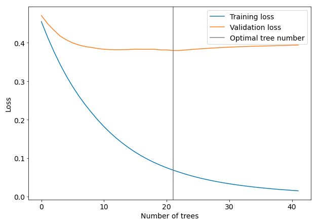
As you can see from the plot the optimal number of tree was selected exactly before the loss values started to increase on validation dataset. The training was stopped. We set n_estimators=100 but only 42 trees were trainined. The optimal numer of trees is 22. We can check the optimal number of trees by printing the best_iteration value:
model.best_iteration

# results
> 22
To compute the predictions we use predict() method, we can pass ntree_limit argument, but in the case of Scikit-Learn API of Xgboost it is not needed. Both versions predict(X) and predict(X, iteration_range=(0, model.best_iteration+1)) return the same values:
model.predict(X_test)

# result
> array([0.93680346, 0.04154444, 0.9282346 , 0.84900916, 0.0657784 ,
       0.92436266, 0.63648796, 0.9468495 , 0.2629984 , 0.9504917 ,
       0.04154444, 0.84900916, 0.89390475, 0.9255801 , 0.04154444,
       0.07570445, 0.92072046, 0.07966585, 0.9510616 , 0.9365885 ,
       0.84900916, 0.07545377, 0.9308903 , 0.9200338 , 0.0657784 ],
      dtype=float32)
Set iteration_range in the predict() (which means that you select how many trees from model should be used to compute predictions):
model.predict(X_test, iteration_range=(0, model.best_iteration+1))

# result
> array([0.93680346, 0.04154444, 0.9282346 , 0.84900916, 0.0657784 ,
       0.92436266, 0.63648796, 0.9468495 , 0.2629984 , 0.9504917 ,
       0.04154444, 0.84900916, 0.89390475, 0.9255801 , 0.04154444,
       0.07570445, 0.92072046, 0.07966585, 0.9510616 , 0.9365885 ,
       0.84900916, 0.07545377, 0.9308903 , 0.9200338 , 0.0657784 ],
      dtype=float32)
To save and load model you can simply run:
# save
model.save_model("my_xgboost.json")

# load
new_model = xgb.XGBRegressor()
new_model.laod_model("my_xgboost.json")

# check optimal number of trees of loaded model
new_model.best_iteration

# result
> 22
Conclusions
The Scikit-Learn API fo Xgboost python package is really user friendly. You can easily use early stopping technique to prevent overfitting, just set the early_stopping_rounds argument when constructin Xgboost object. I usually use 50 rounds for early stopping with 1000 trees in the model. I've seen in many places recommendation to use about 10% of total number of trees for early stopping - such recommendation sounds reasonable. With Scikit-Learn API of Xgboost you don't need to worry about selecting optimal number of tree during predict() and save and load of the model.
AI Data Analyst on Your Computer
Use MLJAR Studio to explore data, find insights, and create reports with AI. Everything runs locally, so your data stays with you.
About the Author

Related Articles
- AutoML in the Notebook
- How does AutoML work?
- Machine Learning for Lead Scoring
- MLJAR AutoML adds integration with Optuna
- How to save and load Xgboost in Python?
- CatBoost with custom evaluation metric
- The next-generation of AutoML frameworks
- MLJAR Studio a new way to build data apps
- Read Google Sheets in Python with no-code MLJAR Studio
- How to authenticate Python to access Google Sheets with Service Account JSON credentials