Tensorflow vs Scikit-learn

Have you ever wonder what is the difference between Tensorflow and Sckit-learn? Which one is better? Have you ever needed Tensorflow when you already use Scikit-learn?

Both packages are from the Machine Learning world. The Tensorflow is a library for differentiable programming. It allows constructing Machine Learning algorithms such as Neural Networks. It is used in Deep Learning. It was developed by Google. At the time of writing, its GitHub repository has 149k stars.

The Scikit-learn is a library that contains ready algorithms for Machine Learning, which can be used to solve tasks like: classification, regression, clustering. It has also a set of methods for data preparation. It was designed to cooperate with packages like NumPy, SciPy, Pandas, Matplotlib. Its GitHub repository has 42.5k stars.

The Tensorflow was designed to construct Deep Neural Networks which can work with various data formats: tabular data, images, text, audio, videos. On the other hand, the Scikit-learn is rather for the tabular data.

Multi Layer Perceptron

In the case of tabular data, a popular architecture of Neural Network (NN) is a Multi-Layer Perceptron (MLP). In Tensorflow you can, of course, build almost any type of NN. The interesting fact is that the MLP algorithm is also available in Scikit-learn. There are available two algorithms:

• for classification: MLPClassifier
• for regression: MLPRegressor

Let's compare them with Tensorflow! :)

The implmentation of MLP Neural Network with Keras and Tensorflow

In the comparison, I will use simple MLP architecture with 2 hidden layers and Adam optimizer.

To use Tensorflow, I will use Keras which provides higher-level API abstraction with ready NN layers.

The code to construct the MLP with Tensorflow and Keras (TF version == 2.2.0, Keras version == 2.3.1):

# data iformation
input_dim = 12 # number of input features
number_of_classes = 3 # number of classes
ml_task = "multiclass_classification" # task that we are going to solve
# initial hyperparameters
dense_1_size = 32
dense_2_size = 16
learning_rate = 0.05

# define model architecture
model = Sequential()
model.add(Dense(dense_1_size, activation="relu", input_dim=input_dim))
model.add(Dense(dense_2_size, activation="relu"))
if ml_task == "multiclass_classification":
    model.add(Dense(number_of_classes, activation="softmax"))
elif ml_task == "binary_classification":
    model.add(Dense(1, activation="sigmoid"))
else: # regression
    model.add(Dense(1))

# compile the model
opt = Adam(learning_rate=learning_rate)
if ml_task == "multiclass_classification":
    model.compile(optimizer=opt, loss="categorical_crossentropy")
elif ml_task == "binary_classification":
    model.compile(optimizer=opt, loss="binary_crossentropy")
else: # regression
    model.compile(optimizer=opt, loss="mean_squared_error")

And the code to train the MLP with early stopping on 10% of the train data:

# X and y are training data

batch_size = min(200, X.shape[0])
epochs = 500
      
stratify = y if ml_task != "regression" else None
X_train, X_vald, y_train, y_vald = train_test_split(
    X, y, test_size=0.1, shuffle=True, stratify=stratify
)
# set callbacks
es = EarlyStopping(monitor="val_loss", mode="min", verbose=0, patience=10)
mc = ModelCheckpoint(
    "best_model.h5",
    monitor="val_loss",
    mode="min",
    verbose=0,
    save_best_only=True,
)

model.fit(
    X_train,
    y_train,
    validation_data=(X_vald, y_vald),
    batch_size=batch_size,
    epochs=500,
    verbose=False,
    callbacks=[es, mc],
)

The implementation of the MLP Neural Network with Scikit-learn

The Scikit-learn version == 0.23.2. The code to create the model:

# initial hyperparameters
dense_1_size = 32
dense_2_size = 16
learning_rate = 0.05
epochs = 500 

# the model
model = MLPClassifier(
    hidden_layer_sizes=(dense_1_size, dense_2_size),
    activation="relu",
    solver="adam",
    learning_rate="constant",
    learning_rate_init=learning_rate, 
    early_stopping=True,
    max_iter=epochs
)

If you need the MLP for regression just change the MLPClassifier to MLPRegressor.

The code to train the model:

# X and y are training data
model.fit(X, y)

That's all! As you can see, you need much more code with Tensorflow+Keras - it is a much flexible library in terms of constructing Neural Networks and that's why you need to define the whole architecture by yourself. The implementation of MLP from Scikit-learn is more like an off-the-shelf algorithm.

Let's take some data!

I get the data for comparison from Penn Machine Learning Benchamrks. They have a lot of example datasets there. I considered only datasets with 1k or more rows. The methodology of comparison was simple:

• take the dataset, split it, 75% of data is used for training and 25% for testing,
• train different Neural Networks architectures, and select the best one (based on 5-fold cross-validation on train data), use the best model to compute predictions on test samples,
• the data preparation (converting categoricals, target scaling in regression) is handled by AutoML mljar-supervised,
• the hyperparameters tuning is handled by AutoML mljar-supervised,
• for classification, I've used logloss and for regression mean squared error metrics.

I used below set of hyperparameters for both implementations of MLP:

nn_params = {
    "dense_1_size": [16, 32, 64],
    "dense_2_size": [4, 8, 16, 32],
    "learning_rate": [0.01, 0.05, 0.08, 0.1],
}

The AutoML was drawing values of hyperparameters from the defined set. A model was skipped, if the drawn values were repeated. There were trained up to 13 different Neural Networks for each implementation for each dataset.

The classification task

There were used 66 datasets in classification (both binary and multiclass). The results are reported in the table below. The time reported is in seconds - it is a total time used for checking all drawn architectures.

Dataset	nrows	ncols	classes	Sklearn_logloss	TF_logloss	Sklearn_time	TF_time
Epistasis_2_1000atts_0.4H	1600	1000	2	0.692272	0.693278	111.71	140.36
Epistasis_2_20atts_0.1H	1600	20	2	0.69291	0.694732	27.42	111.56
Epistasis_2_20atts_0.4H	1600	20	2	0.654114	0.666128	20.41	95.89
Epistasis_3_20atts_0.2H	1600	20	2	0.69219	0.693055	18.5	97.85
Heterogeneity_50	1600	20	2	0.662284	0.692669	24.51	102.42
Heterogeneity_75	1600	20	2	0.685651	0.684641	22.04	150.61
Hill_Valley_with_noise	1212	100	2	0.701181	0.679262	23.4	183.42
Hill_Valley_without_noise	1212	100	2	0.693029	0.693106	22.19	151.83
adult	48842	14	2	0.31302	0.308794	225.9	529.94
agaricus_lepiota	8145	22	2	0.000476217	1.28456e-08	74.34	1417.37
allbp	3772	29	3	0.105024	0.0873737	24.18	261.19
allhyper	3771	29	4	0.0543183	0.0540823	40.24	239.92
allhypo	3770	29	3	0.15851	0.182609	36.58	300.35
allrep	3772	29	4	0.0965378	0.0877159	33.73	289.45
ann_thyroid	7200	21	3	0.0663306	0.0522971	118.12	281.09
car	1728	6	4	0.0565009	0.0270733	25.95	336.2
car_evaluation	1728	21	4	0.0355119	0.0162453	26.77	364.57
chess	3196	36	2	0.0381836	0.0262048	36.16	433.17
churn	5000	20	2	0.232703	0.233059	45.63	342.09
clean2	6598	168	2	0.00358971	1.72954e-05	106.99	1065.38
cmc	1473	9	3	0.872536	0.865697	12.78	255.28
coil2000	9822	85	2	0.206189	0.205792	103.68	394.26
connect_4	67557	42	3	0.454379	0.449654	874.97	1194.23
contraceptive	1473	9	3	0.872536	0.864501	13.88	284.1
credit_g	1000	20	2	0.54315	0.539984	19.76	310.27
dis	3772	29	2	0.0700903	0.0487778	27.56	325.68
dna	3186	180	3	0.159211	0.149867	45.03	415.93
fars	100968	29	8	0.469888	0.470934	612.58	1017.39
flare	1066	10	2	0.393395	0.388351	21.64	413.38
german	1000	20	2	0.518058	0.521267	35.91	756.61
hypothyroid	3163	25	2	0.0643045	0.0698073	84.57	900.39
kr_vs_kp	3196	36	2	0.048205	0.0500323	29.96	136.31
krkopt	28056	6	18	16.0305	17.489	322.73	438.99
led24	3200	24	10	0.847339	0.852022	28.64	97.79
led7	3200	7	10	0.830557	0.822725	21.63	131.69
letter	20000	16	26	20.9291	20.7423	230.99	263.22
magic	19020	10	2	0.310426	0.307443	172.18	270.02
mfeat_factors	2000	216	10	13.1879	12.7521	40.47	134.59
mfeat_fourier	2000	76	10	5.41445	6.88417	56.89	160.14
mfeat_karhunen	2000	64	10	11.1031	11.0863	30.74	308.79
mfeat_morphological	2000	6	10	6.74621	8.46319	36.51	495.13
mfeat_pixel	2000	240	10	0.105948	0.130936	88.05	534.58
mfeat_zernike	2000	47	10	8.05229	8.27279	45.2	273.91
mnist	70000	784	10	0.106536	0.115172	1844.9	2386.88
mofn_3_7_10	1324	10	2	0.0100037	1.38658e-07	24.3	620.48
mushroom	8124	22	2	0.00113378	2.32726e-08	66.92	1643.03
nursery	12958	8	4	0.00837833	0.00787663	218.48	413.13
optdigits	5620	64	10	0.0614936	0.0626042	58.47	279.3
page_blocks	5473	10	5	0.111967	0.109957	38.02	302.59
parity5+5	1124	10	2	0.366705	0.296488	17.58	347.32
pendigits	10992	16	10	0.0244666	0.0216054	85.26	346.54
phoneme	5404	5	2	0.304275	0.299198	47.83	437.41
poker	1025010	10	10	0.00452098	0.00726474	4062.23	2916.7
ring	7400	20	2	0.0829392	0.0794716	90.69	614.34
satimage	6435	36	6	0.242709	0.22644	63.6	365.15
segmentation	2310	19	7	0.118182	0.110797	34.36	313.02
shuttle	58000	9	7	0.00396879	0.00399241	254.09	783.73
sleep	105908	13	5	0.63446	0.62662	412.82	1260.44
solar_flare_2	1066	12	6	0.567718	0.549793	23.22	454.14
spambase	4601	57	2	0.164812	0.162715	55.17	511.57
splice	3188	60	3	0.314676	0.365399	46.27	309.57
texture	5500	40	11	15.8874	20.6093	58.74	573.67
twonorm	7400	20	2	0.0600894	0.0581619	46.37	717.49
waveform_21	5000	21	3	0.293883	0.297824	45.55	544.52
waveform_40	5000	40	3	0.290914	0.291565	47.11	536.87
wine_quality_red	1599	11	6	0.930231	0.954956	34.55	437.98

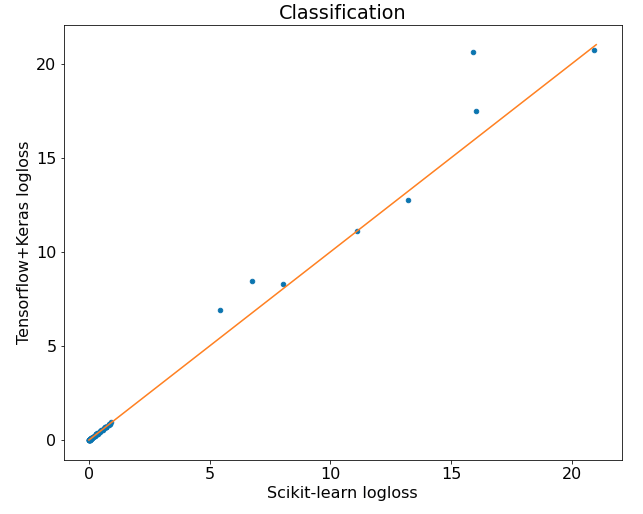
The results can be plotted as scatter plot:

Let's zoom to the [0,1] range:

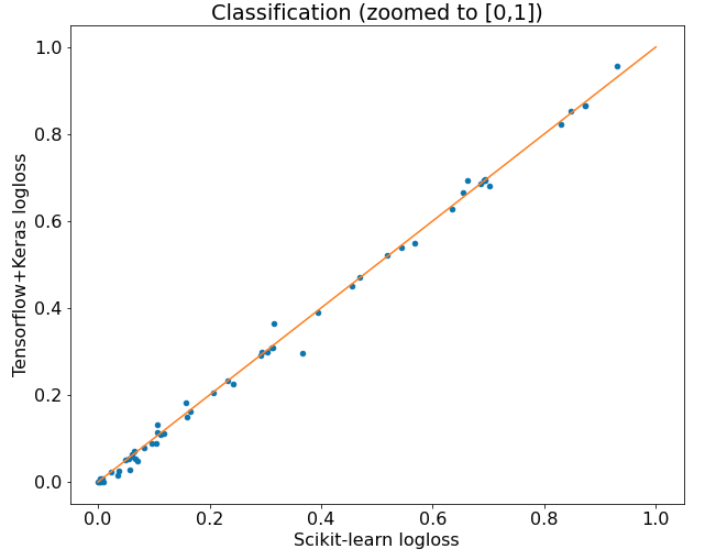
There were 66 datasets and the Tensorflow implementation was 39 times better than Scikit-learn implementation. The differences weren't huge.

It's worth to take a look at times of computation. All computations were on the CPU. The mean time of computation for Scikit-learn was 177 seconds while for Tensorflow it was 508 seconds. The Scikit-learn is much faster. Maybe because TF is intended to be used on GPU rather than CPU? I don't know.

The regression task

There were 48 datasets in the regression task. The results are in the table below:

Dataset	nrows	ncols	Scikit_MSE	TF_MSE	Scikit_time	TF_time
1028_SWD	1000	10	0.351288	0.350476	16.9	84.53
1029_LEV	1000	4	0.404629	0.398672	19.1	64.97
1030_ERA	1000	4	2.51881	2.5505	17.34	92.35
1191_BNG_pbc	1000000	18	688631	688662	3567.38	3557.82
1193_BNG_lowbwt	31104	9	207709	208230	135.2	224.09
1196_BNG_pharynx	1000000	10	85241.6	85288.7	3562.32	3290.37
1199_BNG_echoMonths	17496	9	135.59	135.655	86.55	152.94
1201_BNG_breastTumor	116640	9	91.819	91.538	416.2	879.4
1203_BNG_pwLinear	177147	10	7.64677	7.64574	431.18	874.16
1595_poker	1025010	10	0.0828265	0.0928364	3371.3	3165.36
197_cpu_act	8192	21	6.04194	6.18341	102.1	197.32
201_pol	15000	48	6.82901	6.484	128.53	220.26
215_2dplanes	40768	10	1.00462	1.00613	149.9	395.09
218_house_8L	22784	8	7.6172e+08	7.66826e+08	153.39	389.73
225_puma8NH	8192	8	10.2505	10.3683	39.81	255.74
227_cpu_small	8192	12	7.90558	8.14906	47.62	295.11
294_satellite_image	6435	36	0.490969	0.482076	79.77	324.38
344_mv	40768	10	0.00101928	0.00076863	191.04	563.72
4544_GeographicalOriginalofMusic	1059	117	0.274018	0.252322	24.36	212.47
503_wind	6574	14	9.51609	9.43174	35.83	337.39
529_pollen	3848	4	2.00028	1.98782	20.59	320.87
537_houses	20640	8	2.8563e+09	2.78972e+09	130.66	449.33
562_cpu_small	8192	12	7.90558	8.03778	46.5	391.88
564_fried	40768	10	1.06119	1.04008	199.99	648.26
573_cpu_act	8192	21	6.04194	6.11835	97.13	351.69
574_house_16H	22784	16	9.59662e+08	9.6518e+08	172.56	545.2
583_fri_c1_1000_50	1000	50	0.784129	0.767178	20.21	275.6
586_fri_c3_1000_25	1000	25	0.515327	0.645629	18.89	435.76
588_fri_c4_1000_100	1000	100	0.84392	0.917454	18.02	333.99
589_fri_c2_1000_25	1000	25	0.449973	0.572697	20.68	352.22
590_fri_c0_1000_50	1000	50	0.341366	0.373753	23.86	358.61
592_fri_c4_1000_25	1000	25	0.527293	0.618391	19.53	524.52
593_fri_c1_1000_10	1000	10	0.0616339	0.106806	23.56	351.52
595_fri_c0_1000_10	1000	10	0.0737259	0.0729692	15.99	353.94
598_fri_c0_1000_25	1000	25	0.223486	0.234454	22.21	356.71
599_fri_c2_1000_5	1000	5	0.0255253	0.0254379	23.48	376.14
606_fri_c2_1000_10	1000	10	0.0528226	0.0531012	25.89	391.02
607_fri_c4_1000_50	1000	50	0.792365	0.777099	20.87	560.02
608_fri_c3_1000_10	1000	10	0.0529629	0.0580307	25.5	353.62
609_fri_c0_1000_5	1000	5	0.0420409	0.043429	15.71	463.82
612_fri_c1_1000_5	1000	5	0.0313801	0.0311381	24.51	526.56
618_fri_c3_1000_50	1000	50	0.8721	0.881979	18.3	517.28
620_fri_c1_1000_25	1000	25	0.713895	0.748985	15.09	370.89
622_fri_c2_1000_50	1000	50	0.814633	0.876445	21.74	486.49
623_fri_c4_1000_10	1000	10	0.0580734	0.059318	26.21	461.91
628_fri_c3_1000_5	1000	5	0.0664999	0.0591807	19.43	465.6
banana	5300	2	0.287642	0.286359	39.67	741.51
titanic	2201	3	0.662838	0.659142	24.62	719.5

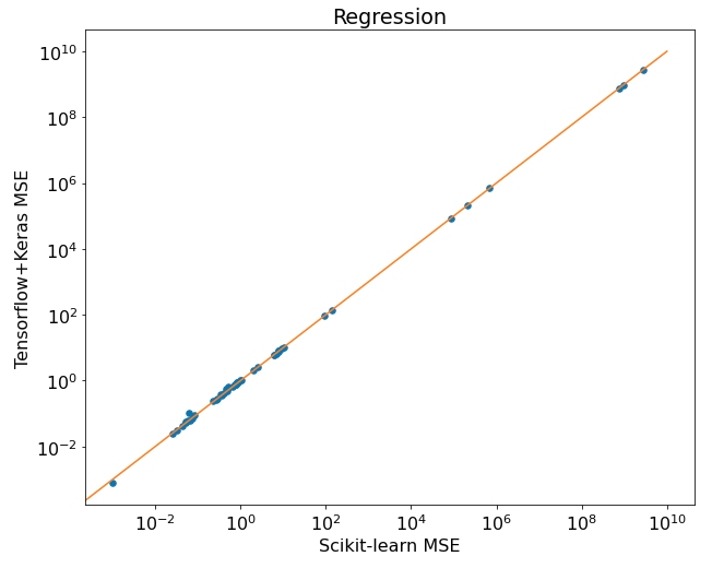
The results can be plotted as scatter plot:

Let's zoom the [0,100] range:

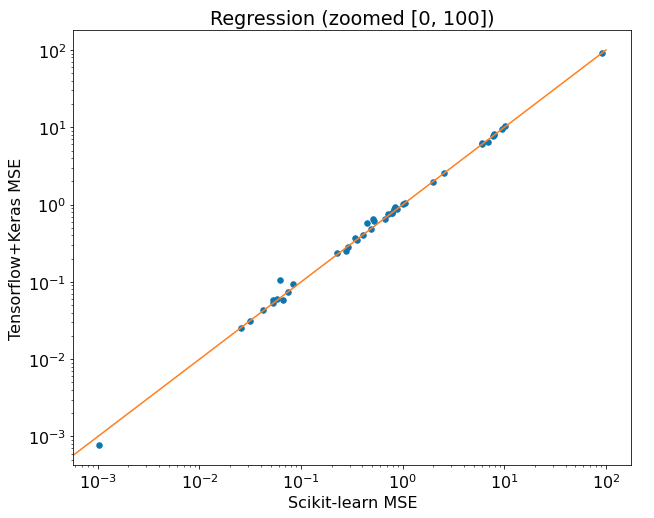
Surprise, surprise! The Scikit-learn MLPRegressor was 28 times out of 48 datasets better than Tensorflow! Again, as in classification, the differences aren't huge. In time comparison, by average it is 286 seconds for Scikit-learn and 586 seconds for Tensorflow.

Summary

• The Tensorflow library is intended to be used to define Deep Neural Networks. All algorithms are defined by the user manually. The high-level packages as Keras can help to speed up the process of NN construction. The library can be used with a variety of data types: tabular, images, text, audio.
• The Scikit-learn package has ready algorithms to be used for classification, regression, clustering ... It works mainly with tabular data.
• When comparing Tensorflow vs Scikit-learn on tabular data with classic Multi-Layer Perceptron and computations on CPU, the Scikit-learn package works very well. It has similar or better results and is very fast.
• When you are using Scikit-learn and need classic MLP architecture, in my opinion, there is no need to grab Tensorflow (which is, by the way, quite a big package over 500MB on PyPi)

---

If you are developing Machine Learning models and want to save time, you definitely should try our AutoML mljar-supervised! It is amazing :)