4 Effective Ways to Visualize XGBoost Trees

XGBoost

XGBoost (eXtreme Gradient Boosting) is a supervised machine learning algorithm that is highly efficient and widely used for both classification and regression tasks. Unlike Random Forest, XGBoost operates by building a sequence of decision trees, where each new tree is trained to correct the errors made by the previous trees. This process is known as boosting, and it results in a more accurate and robust model.

In XGBoost, the algorithm works by constructing multiple decision trees, but instead of training them independently, each tree in the sequence focuses on the mistakes of the earlier trees. The model is updated iteratively, with each tree minimizing the residual errors of the previous ones. The final prediction is a weighted sum of the outputs of all the individual trees. For classification, the model combines the trees’ outputs to assign the sample to a specific class, while for regression, it averages the predicted values.

Each tree in XGBoost is built using gradient descent to optimize the model's performance. This ensures that the trees gradually reduce the error of the overall prediction. Additionally, XGBoost introduces regularization (L1 and L2) to control overfitting, making it more powerful for complex datasets. XGBoost can also handle missing values, sparse data, and large datasets efficiently due to its parallelization and memory-efficient implementation.

XGBoost's key strength lies in its ability to handle noisy or imbalanced datasets and its performance in competitions and real-world applications. Its flexibility and customization options, such as tuning the learning rate, tree depth, and boosting rounds, make it highly effective in improving model accuracy.

The XGBoost algorithm can also be divided into two types based on the target values:

• Classification boosting is used to classify samples into distinct classes, and in scikit-learn, this is implemented using XGBClassifier.
• Regression boosting is used to predict continuous numerical values, and in scikit-learn, this is implemented using XGBRegressor.

XGBoost's ability to provide high accuracy, manage feature importance, and prevent overfitting through regularization has made it a popular choice in data science and machine learning.

Below I show how to use xgboost and 4 ways to plot a tree from it:

• plot_tree - req. matplotlib
• graphviz - req. graphviz
• dtreeviz - req. dtreeviz and graphviz
• supertree - req. supertree

Classification task

Prepare data

I start with preparing my data from iris dataset and splitting it. It will be needed for determining model's accuracy.

# Import necessary libraries
import xgboost as xgb
from sklearn.datasets import load_iris
from sklearn.model_selection import train_test_split
from sklearn.preprocessing import LabelEncoder
from sklearn.metrics import accuracy_score
# Load the Iris dataset
# The dataset contains 150 samples with 4 features and 3 target classes.
iris = load_iris()
X = iris.data  # Features
y = iris.target  # Labels (classes)
features = iris.feature_names  # Feature names
target = 'species'  # Target name for visualization
class_names = iris.target_names  # Class names for visualization
# Split the dataset into training and testing sets
# We'll use 80% of the data for training and 20% for testing.
X_train, X_test, y_train, y_test = train_test_split(X, y_encoded, test_size=0.2, random_state=42)

Train model

I tune hyper-parameter for unified results across the trees.

# Create an XGBClassifier instance
# The classifier uses the same parameters as XGBoost but in a more intuitive way.
xgb_classifier = xgb.XGBClassifier(
    objective='multi:softmax',  # Specify the multi-class classification task
    num_class=3,                # Number of classes (3 in the case of Iris)
    max_depth=5,                # Maximum depth of the trees
    learning_rate=0.3,          # Learning rate for the model
    n_estimators=50,            # Number of boosting rounds (iterations)
    random_state=42             # Set random state for reproducibility
)
# Train the XGBClassifier model
xgb_classifier.fit(X_train, y_train)

# Make predictions on test data
y_pred = xgb_classifier.predict(X_test)

# Output the predictions
print(y_pred)

Model Accuracy: 100.00%

As we see our model scored perfect result. Now it's time to make some plots.

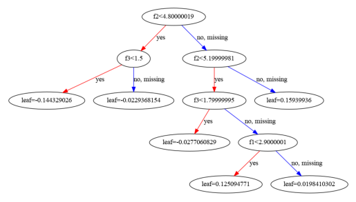
Plot with plot_tree

First method I use comes from xgboost package and to work matplotlib is required. It allows us to easily produce figure of the tree (without intermediate exporting to graphviz). I wrote num_trees=1 to show a second tree.

from xgboost import plot_tree
import matplotlib.pyplot as plt
plt.figure(figsize=(30, 20))  
plot_tree(xgb_classifier, num_trees=1) 
plt.show()

Plot with graphviz

For graphviz method I need to install new package as I hinted before coding. But don't worry, it will be needed in next method too.

For this to work I need to export a tree to a DOT format. I save file and simply display it in notebook.

import graphviz
import os
tree_dot = xgb.to_graphviz(xgb_classifier, num_trees=2)
# Save the dot file
dot_file_path = "xgboost_tree.dot"
tree_dot.save(dot_file_path)
# Convert dot file to png and display
with open(dot_file_path) as f:
    dot_graph = f.read()
# Use graphviz to display the tree
graph = graphviz.Source(dot_graph)
graph.render("xgboost_tree")
# Optionally, visualize the graph directly
graph

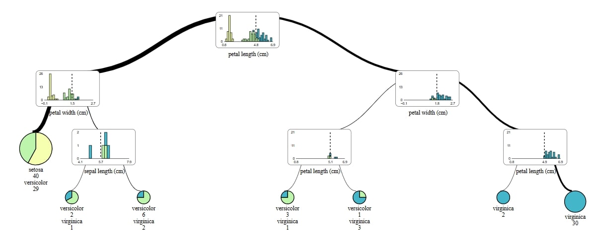
Plot with dtreeviz

The dtreeviz package you can simply install with pip: pip install dtreeviz. Once it installs and our previous graphviz is ready, I can skip step with converting to DOT file.

from dtreeviz import model
viz_model = model(
    xgb_classifier.get_booster(),
    X_train=X_train,
    y_train=y_train,
    feature_names=features,
    target_name=target,
    class_names=list(class_names),
    tree_index=2  # Visualizes the second tree (change this index for other trees)
)
# Display the visualization
viz_model.view()

To save file simply add one line:

viz_model.save()

Plot with supertree

supertree package is our work. It's an interactive plot that allows you to see in detail intricacies of the model. You can use pip to install it with pip install supertree.

from supertree import SuperTree
st = SuperTree(
    xgb_classifier, 
    X_train, 
    y_train, 
    iris.feature_names, 
    iris.target_names
)
# Visualize the tree
st.show_tree(which_tree=2)
#save to html so you could simply open it in browser
#that way you will be able to expand tree, seedetail etc.
st.save_html() 

Regression task

For regression task we use diabetes datatset.

Load data and train model

import xgboost as xgb
from sklearn.datasets import load_diabetes
from sklearn.model_selection import train_test_split
from sklearn.metrics import mean_squared_error

# Load the diabetes dataset
diabetes = load_diabetes()

# Separate features (X) and target (y)
X = diabetes.data  # Features (e.g., age, BMI, etc.)
y = diabetes.target  # Target (a continuous value, which is a measure of disease progression)

# Split the dataset into training and testing sets
# test_size=0.2 means 20% of the data will be used for testing
# random_state ensures reproducibility
X_train, X_test, y_train, y_test = train_test_split(X, y, test_size=0.2, random_state=42)

# Initialize the XGBoost regressor
xgb_regressor = xgb.XGBRegressor(
    objective='reg:squarederror',  # Objective function for regression
    max_depth=5,                   # Maximum depth of each tree
    learning_rate=0.3,             # Step size shrinkage to prevent overfitting
    n_estimators=50,               # Number of trees in the model (boosting rounds)
    random_state=42                # Seed for reproducibility
)

# Train the regressor on the training data
xgb_regressor.fit(X_train, y_train)

All the steps I show from here are very simmiliar to those you could se in Classification Task above. Major differences come only from different datatset and task at hand.

Plot with XGBoost

from xgboost import plot_tree
import matplotlib.pyplot as plt

plt.figure(figsize=(30, 20))  
plot_tree(xgb_regressor, num_trees=2) 
plt.show()

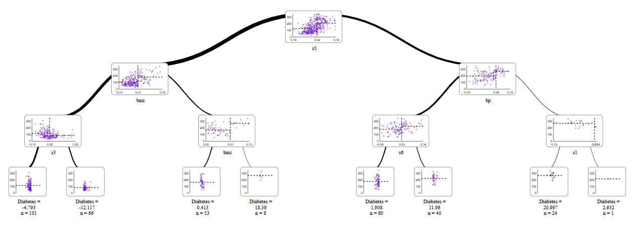
Plot with dtreeviz

from dtreeviz import model

viz_model = model(
    xgb_regressor.get_booster(),
    X_train=X_train,
    y_train=y_train,
    feature_names=diabetes.feature_names,
    target_name="diabetes",
    tree_index=2  
)

viz_model.view()

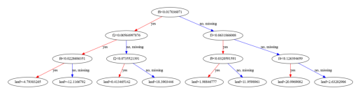
Plot with graphviz

import graphviz
import os

tree_dot = xgb.to_graphviz(xgb_regressor, num_trees=2)

# Save the dot file
dot_file_path = "xgboost_tree.dot"
tree_dot.save(dot_file_path)

# Convert dot file to png and display
with open(dot_file_path) as f:
    dot_graph = f.read()

# Use graphviz to display the tree
graph = graphviz.Source(dot_graph)
graph.render("xgboost_tree")

graph

Plot with supertree

from supertree import SuperTree

st = SuperTree(
    xgb_regressor, 
    X_train, 
    y_train, 
    diabetes.feature_names, 
    "Diabetes"
)
# Visualize the tree
st.show_tree(which_tree=2)

From above methods my favourite is visualizing with supertree package. I like it becuause:

• IT IS INTERACTIVE!
• it shows the distribution of decision feature in the each node
• classes are easily recognisibale
• I can see detail in a node and a leaf
• zoom in and change levels of a tree feature
• by clicking leaf it lights up whole road from start node