4 Effective Ways to Visualize Random Forest

A Random Forest is a supervised algorithm used in machine learning. It operates by constructing a multitude of decision trees (typically using a binary tree structure where each node has two children) and combining their results to improve accuracy and prevent overfitting. In a Random Forest, each data sample is passed through multiple decision trees, each of which assigns a target value to the sample. The final prediction is typically determined by aggregating the outputs of all the individual trees, such as taking the majority vote for classification or averaging the predictions for regression.

The trees in the forest make decisions based on the features of the input sample. Each tree is built independently using a random subset of the data and a random selection of features, which helps to create diversity and reduce correlation between the trees. This process helps to make Random Forest more robust than individual decision trees.

The Random Forest algorithm can be divided into two types based on the target values:

• Classification forests used to classify samples into a set of distinct classes. In scikit-learn, this is handled by the RandomForestClassifier.
• Regression forests used to predict continuous numerical values within a range. In scikit-learn, this is handled by the RandomForestRegressor.

Random Forests are widely used due to their ability to handle large datasets, manage feature importance, and provide high accuracy while reducing overfitting compared to a single decision tree. They are also valuable for decision-making processes because of their ensemble approach and visual interpretability through feature importance and tree visualization.

Below I show how to use scikit-learn and 4 ways to plot a tree from it:

• plot_tree - req. matplotlib
• graphviz - req. graphviz
• dtreeviz - req. dtreeviz and graphviz
• supertree - req. supertree

Classification task

Prepare data

In this example let's use a real classic - iris dataset.

from sklearn.ensemble import RandomForestClassifier
from sklearn.datasets import load_iris
from sklearn.model_selection import train_test_split
from sklearn.metrics import accuracy_score

# Load the Iris dataset
iris = load_iris()

# Separate features (X) and target labels (y)
X = iris.data  # Features (flower measurements)
y = iris.target  # Labels (species)

# Define feature names and target class for clarity
features = iris.feature_names  # List of feature names (petal length, etc.)
target = 'species'  # Target variable (species of the flower)
class_names = iris.target_names  # List of species (setosa, versicolor, virginica)

# Split the dataset into training and testing sets
# test_size=0.2 means 20% of the data will be used for testing
# random_state ensures reproducibility
X_train, X_test, y_train, y_test = train_test_split(X, y, test_size=0.2, random_state=42)

Train model

# Initialize the RandomForestClassifier
rf_classifier = RandomForestClassifier(
    n_estimators=50,  # Number of trees in the forest
    max_depth=5,      # Maximum depth of the trees
    random_state=42   # Seed for reproducibility
)

# Train the classifier on the training data
rf_classifier.fit(X_train, y_train)

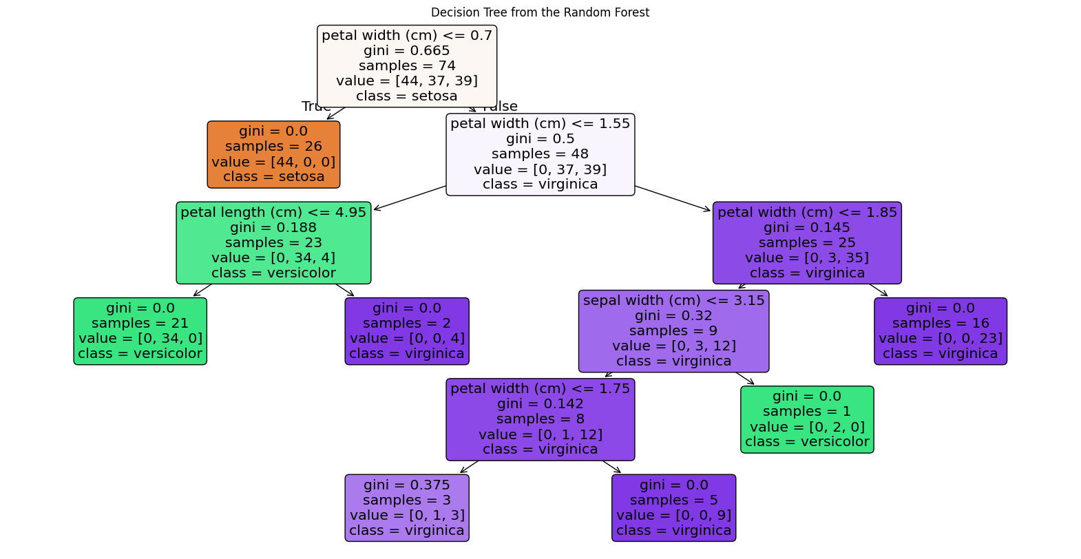
Plot with plot_tree

First method I use comes from sklearn package and to work matplotlib is required. It allows us to easily produce figure of the tree (without intermediate exporting to graphviz).

import matplotlib.pyplot as plt
from sklearn.tree import plot_tree
# Plot the tree using the plot_tree function from sklearn
tree = rf_classifier.estimators_[0]
plt.figure(figsize=(20,10))  # Set figure size to make the tree more readable
plot_tree(tree, 
          feature_names=features,  # Use the feature names from the dataset
          class_names=class_names,  # Use class names (species names)
          filled=True,              # Fill nodes with colors for better visualization
          rounded=True)             # Rounded edges for nodes
plt.title("Decision Tree from the Random Forest")
plt.show()

Plot with graphviz

graphviz outpur may look simmilar to plot_tree() but is more readable. Additional work that needs to be done is exporting my tree to a DOT file.

from sklearn.tree import export_graphviz
import graphviz

# Assuming rf_classifier is already trained
# Select one tree from the random forest (e.g., the first one)
tree = rf_classifier.estimators_[0]

# Export the selected tree to DOT format
dot_file_path = "random_forest_tree.dot"
export_graphviz(
    tree, 
    out_file=dot_file_path, 
    feature_names=features,  # Feature names from the Iris dataset
    class_names=class_names,  # Class names (setosa, versicolor, virginica)
    filled=True,  # Color the nodes
    rounded=True,  # Rounded corners for nodes
    special_characters=True  # Allows special characters in labels
)

with open(dot_file_path) as f:
    dot_graph = f.read()

# Visualize the tree using graphviz
graph = graphviz.Source(dot_graph)
graph.render("random_forest_tree")
graph  # Display the tree graph

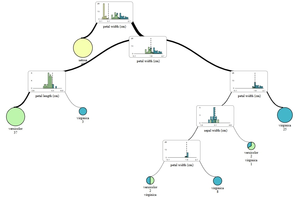
Plot with dtreeviz

To use dtreeviz don't forget to install graphviz. With it I not only skip converting tree, but also it creates diagrams within plot. Plots made with dtreeviz are elegant and insightful.

from dtreeviz import model
tree = rf_classifier.estimators_[0]

viz_model = model(
    tree,
    X_train=X_train,
    y_train=y_train,
    target_name=target,
    class_names=list(class_names),
    tree_index=2  
)

viz_model.view()

Plot with supertree

supertree is single INTERACTIVE package on my list of ways to visualize tree from random forests.

It's easy to use and in my humnle opinion is the most visually appealing out of all 4 packages.

from supertree import SuperTree

st = SuperTree(
    rf_classifier, 
    X_train, 
    y_train, 
    iris.feature_names, 
    iris.target_names
)

st.show_tree(which_tree=0)

Regression

For regression task I'm going to use diabetes data.

Becuase this examples are very simmilar, I will limit myself to comments in code.

Train model

from sklearn.ensemble import RandomForestRegressor
from sklearn.datasets import load_diabetes
from sklearn.model_selection import train_test_split
from sklearn.tree import export_graphviz
import graphviz

# Load the diabetes dataset
diabetes = load_diabetes()

# Separate features (X) and target (y)
X = diabetes.data  # Features (e.g., age, BMI, etc.)
y = diabetes.target  # Target (a continuous value, which is a measure of disease progression)

# Split the dataset into training and testing sets
X_train, X_test, y_train, y_test = train_test_split(X, y, test_size=0.2, random_state=42)

# Initialize the RandomForestRegressor
rf_regressor = RandomForestRegressor(
    n_estimators=50,  # Number of trees in the forest
    max_depth=5,      # Maximum depth of the trees
    random_state=42   # Seed for reproducibility
)

# Train the regressor on the training data
rf_regressor.fit(X_train, y_train)

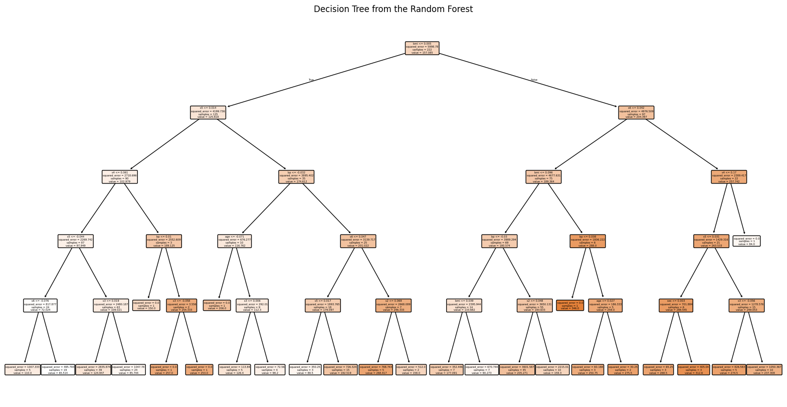
Plot with plot_tree

import matplotlib.pyplot as plt
from sklearn.tree import plot_tree

# Assuming rf_regressor is a trained RandomForestRegressor
tree = rf_regressor.estimators_[0]

# Load the diabetes dataset
diabetes = load_diabetes()

# Set figure size
plt.figure(figsize=(20, 10))

# Plot the tree
plot_tree(tree, 
          feature_names=diabetes.feature_names,  # Use the feature names from the dataset
          filled=True,              # Fill nodes with colors for better visualization
          rounded=True)             # Rounded edges for nodes

# Add a title
plt.title("Decision Tree from the Random Forest")
plt.show()

Plot with graphviz

tree = rf_regressor.estimators_[0]

# Define feature names (the diabetes dataset does not provide feature names directly)
features = diabetes.feature_names
# Export the selected tree to DOT format
dot_file_path = "diabetes_forest_tree.dot"
export_graphviz(
    tree, 
    out_file=dot_file_path, 
    feature_names=features,  # Feature names from the diabetes dataset
    filled=True,  # Color the nodes
    rounded=True,  # Rounded corners for nodes
    special_characters=True  # Allows special characters in labels
)

# Read the DOT file and visualize the tree using Graphviz
with open(dot_file_path) as f:
    dot_graph = f.read()

# Visualize the tree using graphviz
graph = graphviz.Source(dot_graph)
graph.render("diabetes_forest_tree")  # Save the tree visualization as a file
graph

Plot with dtreeviz

from dtreeviz import model
tree = rf_regressor.estimators_[0]

viz_model = model(
    tree,
    X_train=X_train,
    y_train=y_train,
    feature_names=diabetes.feature_names,
    target_name="diabetes",
)

viz_model.view()

Plot with supertree

In previous example tree is a little unreadable. supertree has simmilar problem, but fixes it. I can use scroll in my mouse to zoom in on particular elements and see details on interactive diagrams.

You can try this out on mljar.com/supertree.

from supertree import SuperTree

st = SuperTree(
    rf_regressor, 
    X_train, 
    y_train, 
    diabetes.feature_names, 
    "diabetes"
)

st.show_tree(which_tree=0)

supertree package looks like great all-rounder, especially in notebooks. It not only looks interesting but also gives easy acces to details by hovering mouse over elements. However I think that this interactivity is what rises supertree over other comeptitors.

I can not recommed this package enough.