4 Effective Ways to Visualize LightGBM Trees

LightGBM

LightGBM (Light Gradient Boosting Machine) is a powerful supervised machine learning algorithm designed for efficient performance, especially on large datasets. Similar to XGBoost, it is used for both classification and regression tasks, but LightGBM offers faster training speed and lower memory usage by leveraging a leaf-wise tree growth strategy. This method splits the leaf with the highest potential for error reduction, leading to deeper trees and better accuracy than level-wise tree growth used by traditional methods like Random Forest.

LightGBM builds a sequence of decision trees, where each new tree corrects the errors of the previous ones in a process known as boosting. This iterative training helps the model become more accurate over time. Each tree's contribution is a weighted adjustment to the overall prediction. For classification, the final output assigns a class based on the combined predictions, while for regression, it outputs an averaged value.

The algorithm uses gradient descent to minimize the residual errors of earlier trees, improving model performance iteratively. LightGBM also implements L1 and L2 regularization, helping control overfitting and making it highly effective for complex datasets. Additionally, LightGBM is designed to handle missing values and sparse data, and it scales efficiently for large datasets thanks to its parallel and memory-optimized implementation.

LightGBM’s strength lies in its speed and efficiency, especially with large-scale data, imbalanced datasets, or high-dimensional features. Its flexible parameters allow tuning of hyperparameters like the learning rate, tree depth, and number of boosting iterations, making it an ideal choice for high-performance machine learning tasks.

LightGBM can be categorized into two types based on the target values:

• Classification boosting for categorizing data into distinct classes. In scikit-learn, this can be done using LGBMClassifier.
• Regression boosting for predicting continuous numerical values. In scikit-learn, this can be done using LGBMRegressor.

Below, I show how to use lightgbm and 4 ways to visualize its decision trees:

• plot_tree – requires matplotlib
• graphviz – requires graphviz
• dtreeviz – requires dtreeviz and graphviz
• supertree – requires supertree

Classification

Prepare data nad train model

For showcases like this I like using well known data and every single one data scientist used 'iris' dataset.

After splitting dataset we tune parameters and start training a model.

import lightgbm as lgb
from sklearn.datasets import load_iris
from sklearn.model_selection import train_test_split
from sklearn.metrics import accuracy_score

# Load the Iris dataset
# X: features (sepal length, sepal width, petal length, petal width)
# y: target labels (species of iris flowers)
iris = load_iris()
X = iris.data  # Feature matrix
y = iris.target  # Target vector (species)
features = iris.feature_names  # Names of the features
target = 'species'  # Target label name
class_names = iris.target_names  # Names of the target classes (species)

# Split the dataset into training and test sets
# 80% training data, 20% test data
X_train, X_test, y_train, y_test = train_test_split(X, y, test_size=0.2, random_state=42)

# Create a LightGBM classifier
lgb_classifier = lgb.LGBMClassifier(
    objective='multiclass',  # Specifies the objective for multi-class classification
    num_class=3,             # Number of classes (3 species in the Iris dataset)
    max_depth=5,             # Maximum depth of each tree (prevents overfitting)
    learning_rate=0.3,       # Learning rate (controls how quickly the model adapts to the data)
    n_estimators=50,         # Number of boosting rounds (number of trees in the model)
    random_state=42,          # Seed for reproducibility
    verbose=-1
)

# Fit the model to the training data
# This trains the classifier using the training set (X_train, y_train)
lgb_classifier.fit(X_train, y_train)

Visualize with LGBM

lightgbm package contains method to convert data, but to display it I need matplotlib.

import lightgbm as lgb
import matplotlib.pyplot as plt

plt.figure(figsize=(30, 20))
ax = lgb.plot_tree(lgb_classifier, tree_index=0, figsize=(30, 20), show_info=['split_gain', 'internal_value', 'leaf_count'])
plt.show()

With tree_index=0 choose first tree and in show_info=[] I can decide what labels I wanna use in this plot.

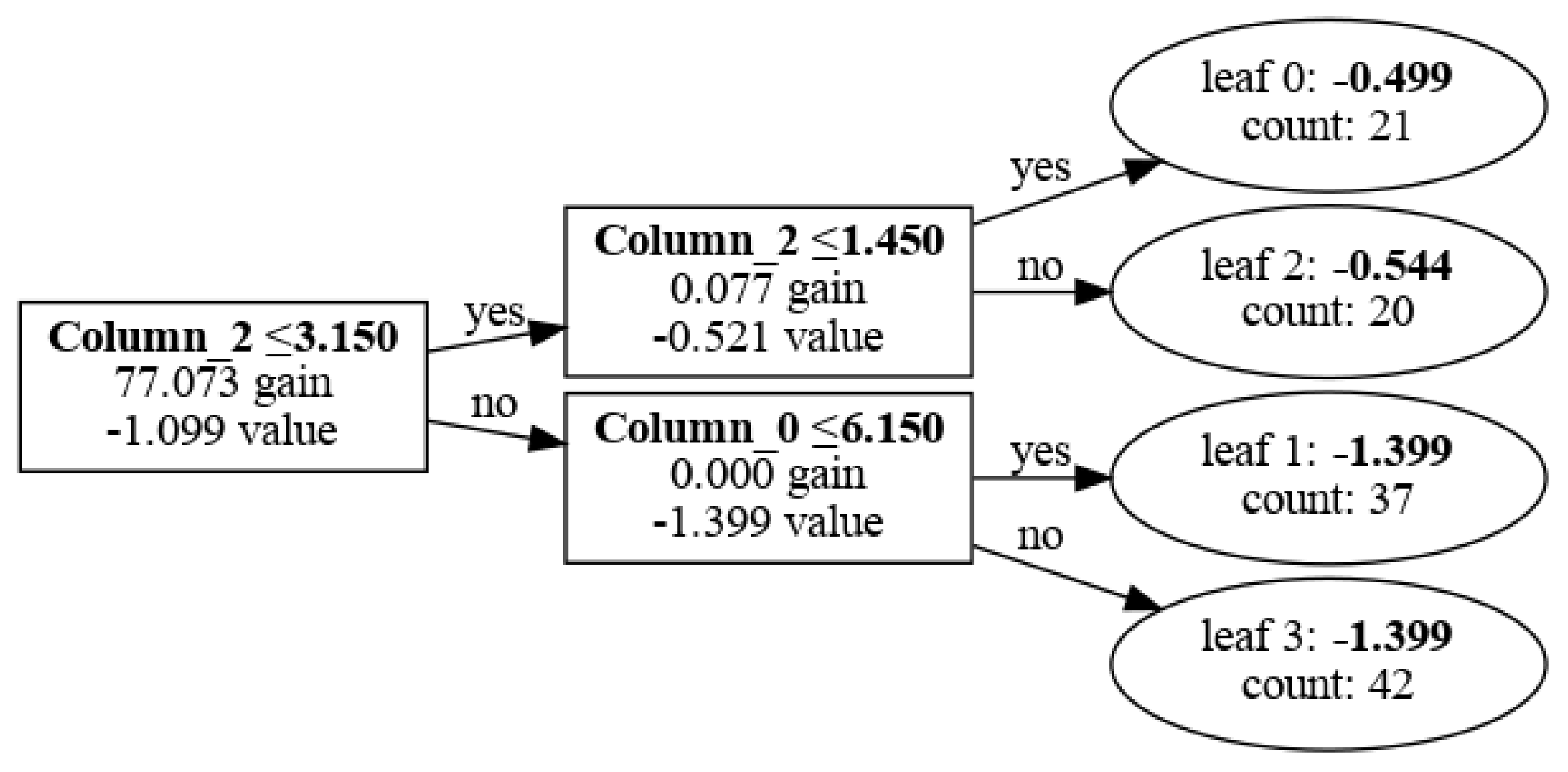
Visualize with graphviz

graphviz developers had different approach. With this package we plot from raw LightGBM model. Before we can plot tree, DOT file is generated of a chosen tree. Then I can convert tree structure to PNG file and display it.

import graphviz
import os
# Extract the booster (raw model) from the LightGBM classifier
booster = lgb_classifier.booster_

# Generate the DOT format for a specific tree (e.g., tree 2)
tree_dot = booster.dump_model()["tree_info"][2]  # Extract the third tree (index starts from 0)

# Convert tree structure to DOT format
dot_data = lgb.create_tree_digraph(booster, tree_index=2)

# Save the dot file
dot_file_path = "lgbm_tree.dot"
with open(dot_file_path, "w") as f:
    f.write(dot_data.source)

# Use Graphviz to display the tree
graph = graphviz.Source(dot_data.source)
graph.render("lgbm_tree")

graph

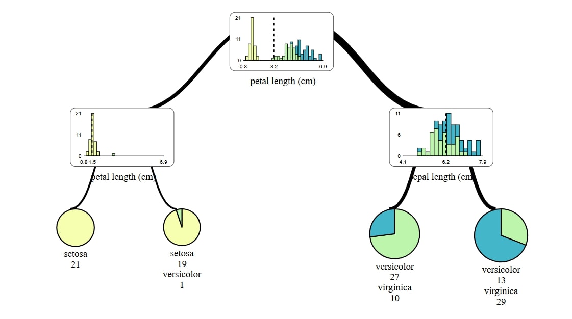
Visualize with dtreeviz

For using dtreeviz it requires of course its own, but also a graphviz package. With dtreeviz I not only don't need to generate and convert files, but also final view is much more pleasing thanks to added automatically colors.

from dtreeviz import model
booster = lgb_classifier.booster_

viz_model = model(
    booster,
    X_train=X_train,
    y_train=y_train,
    feature_names=features,
    target_name=target,
    class_names=list(class_names),
    tree_index=0  
)

viz_model.view()

To save file simply add viz_model.save() with name of file, ex. classification.svg

Visualize with SuperTree

With supertree we can elevate visualisation of decission trees. All thanks to interactive abilities of our package.

from supertree import SuperTree

st = SuperTree(
    lgb_classifier, 
    X_train, 
    y_train, 
    iris.feature_names, 
    iris.target_names
)
# Visualize the tree
st.show_tree(which_tree=0)

supertree even can change tree in forest dynamicaly in notepads. Simply change last lines to:

# Turn on the feature
# Visualize the tree
st.show_tree(widget=true, which_tree=0)

Regression

iris dataset is not suitable for regression task so I change it to diabetes dataset.

Most of steps are very simmilar to those in classification.

Prepare data nad train model

import lightgbm as lgb
from sklearn.datasets import load_diabetes
from sklearn.model_selection import train_test_split
from sklearn.metrics import mean_squared_error

# Load the Diabetes dataset
# X: features (numerical variables that may impact diabetes progression)
# y: target (quantitative measure of disease progression after one year)
diabetes = load_diabetes()
X = diabetes.data  # Feature matrix
y = diabetes.target  # Target vector (disease progression measure)

# Split the dataset into training and test sets
# 80% training data, 20% test data
X_train, X_test, y_train, y_test = train_test_split(X, y, test_size=0.2, random_state=42)

# Create a LightGBM regressor model
lgb_regressor = lgb.LGBMRegressor(
    objective='regression',  # Regression problem
    max_depth=5,             # Restricting the maximum depth of the trees to prevent overfitting
    learning_rate=0.1,       # Learning rate controls the step size during gradient boosting
    n_estimators=100,        # Number of boosting iterations (number of trees)
    random_state=42          # Seed for reproducibility
)

# Train the model on the training data
# This fits the model to the data by building decision trees with boosting
lgb_regressor.fit(X_train, y_train)

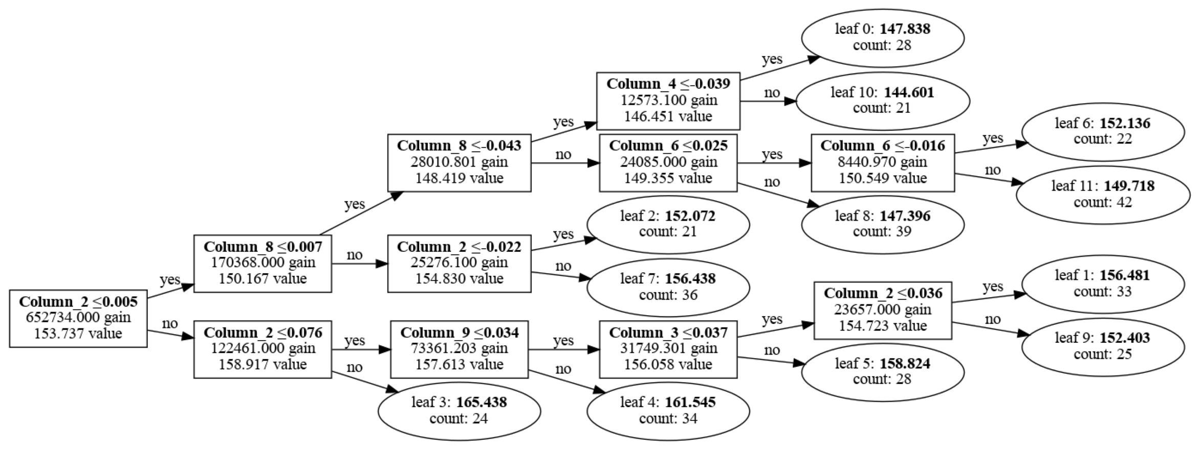
Visualize with LGBM

import lightgbm as lgb
import matplotlib.pyplot as plt

plt.figure(figsize=(30, 20))
ax = lgb.plot_tree(lgb_regressor, tree_index=0, figsize=(30, 20), show_info=['split_gain', 'internal_value', 'leaf_count'])
plt.show()

Visualize with graphviz

import graphviz
import os
# Extract the booster (raw model) from the LightGBM classifier
booster = lgb_regressor.booster_

# Generate the DOT format for a specific tree (e.g., tree 2)
tree_dot = booster.dump_model()["tree_info"][2]  # Extract the third tree (index starts from 0)

# Convert tree structure to DOT format
dot_data = lgb.create_tree_digraph(booster, tree_index=0)

# Save the dot file
dot_file_path = "lgbm_tree.dot"
with open(dot_file_path, "w") as f:
    f.write(dot_data.source)

# Use Graphviz to display the tree
graph = graphviz.Source(dot_data.source)
graph.render("lgbm_tree")

graph

Visualize with dtreeviz

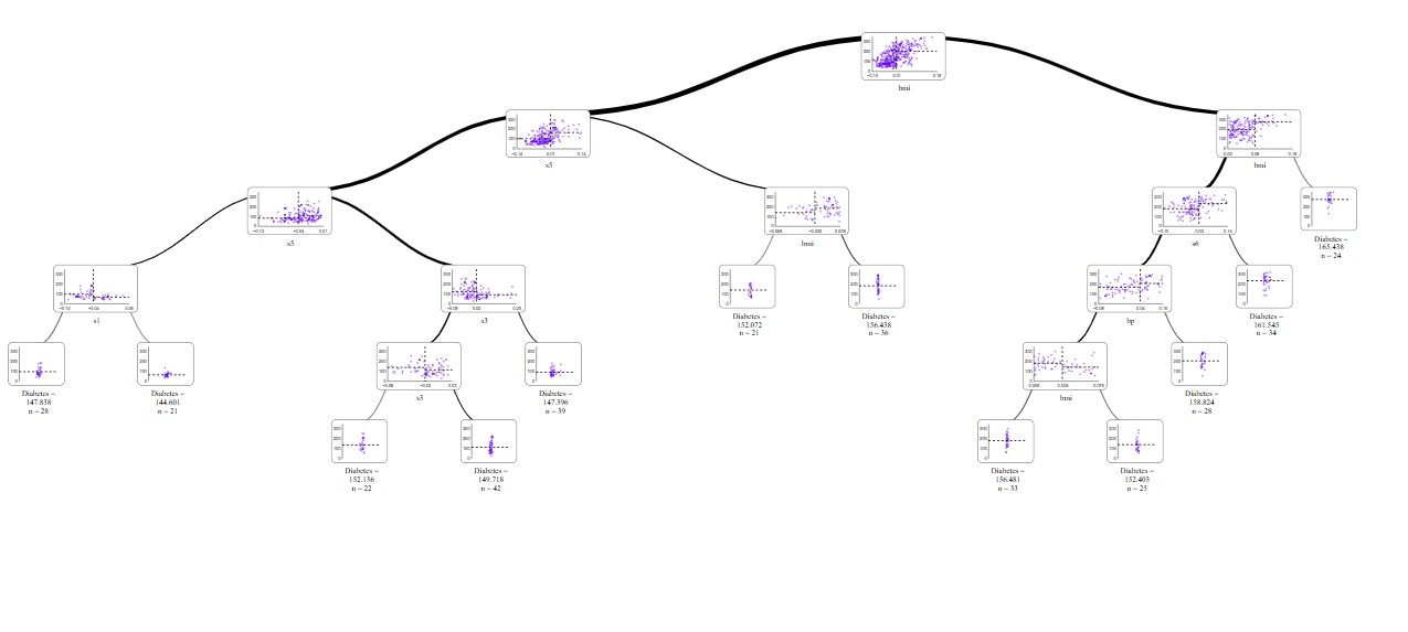
from dtreeviz import model
booster = lgb_regressor.booster_

viz_model = model(
    booster,
    X_train=X_train,
    y_train=y_train,
    feature_names=diabetes.feature_names,
    target_name="Diabetes",
    tree_index=0  
)

viz_model.view()

Visualize with SuperTree

from supertree import SuperTree

st = SuperTree(
    lgb_regressor, 
    X_train, 
    y_train, 
    diabetes.feature_names, 
    "Diabetes"
)
# Visualize the tree
st.show_tree(which_tree=0)

For long time dtreeviz was my go to tool for plots of decision trees but now supertree wins this competition. With interactive tool like supertree researcing and explaining trees became much less of a burden, at least in presentation part.

Interactivity of this package makes it easier to read and understand distribution in nodes, while with zoom in feature it's easy to see details.