My top 10 favorite machine learning algorithms

Machine Learning is the field that focuses on teaching machines (or computer programs) how to learn from data without being explicitly programmed step-by-step. In a traditional programming setup, we tell the computer exactly what to do for every possible situation. However, in Machine Learning, we allow the computer to discover patterns and rules automatically by examining data. This can lead to powerful models that predict or classify new, unseen examples with high accuracy.

In this article, I want to share my favorite Machine Learning algorithms. These algorithms range from simple methods like K-Nearest Neighbors (KNN) to more advanced techniques like Gradient Boosting and Automated Machine Learning (AutoML). Each algorithm has a unique approach to learning, and each one offers different benefits, such as simplicity, speed, interpretability, or accuracy. By understanding the basics of each method, you can decide which algorithm best fits your problem or your preferences.

Below, I present my top 10 algorithms in no particular order. I’ll explain them in a few sentences, provide a simple reason why I enjoy using them. I have also included references to the original research papers and a couple of tools that you can use to implement these algorithms in practice.

1. K-Nearest Neighbors (KNN)

K-Nearest Neighbors was the first algorithm I ever implemented, and I did it using C++. It is very easy to understand because it relies on distances between points in your dataset. You do not need a separate training phase in the usual sense; instead, you store all your training data and then make predictions by finding the nearest neighbors of the test sample. There is a good implementation of kNN algorithm in scikit-learn package, it has a built-in KNeighborsClassifier and KNeighborsRegressor.

How It Works

1. Suppose you have a new data point (for example, a new customer to classify).
2. You look for the K nearest points in your training dataset (based on a distance measure like Euclidean distance) and check their labels (e.g., what category they belong to).
3. The new data point is labeled based on the majority vote among the nearest neighbors (for classification) or some average of their values (for regression).

References

• Cover, T. & Hart, P. (1967). Nearest neighbor pattern classification. IEEE Transactions on Information Theory, 13(1), 21–27.

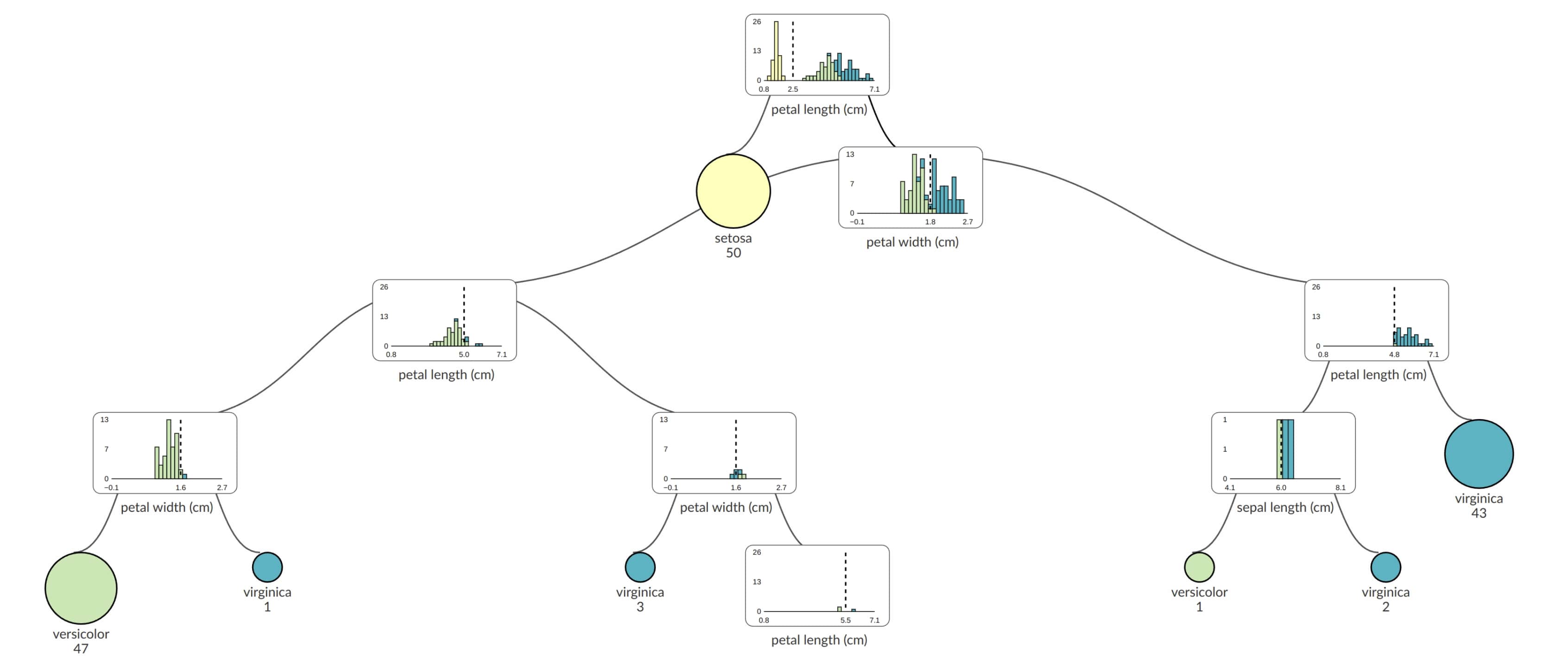
2. Decision Trees

Decision Trees are one of the simplest models to understand. They train quickly, and if you limit the depth (for instance, up to seven levels), they remain compact and easy to interpret. I also appreciate how they can be visually represented as a tree, making it straightforward to see how predictions are made at each split.

The scikit-learn provides implementation of DecisionTreeClassifier and DecisionTreeRegressor. I can recommend supertree open source package for visualizing trained Decision Trees, which I'm co-author. It produces interactive visualization and it works great in the Python notebook.

How It Works

1. The algorithm starts with all your training data in a single group.
2. It then finds a question that splits the data into smaller groups that are as "pure" as possible with respect to the target label (e.g., "Is Age > 30?").
3. This splitting process continues recursively until a stopping criterion is met, and the final leaves give the predictions.

References

• Quinlan, J. R. (1986). Induction of decision trees. Machine Learning, 1(1), 81–106.

3. Random Forest

Do you need better performance than single Decision Tree? Random Forest is like having many Decision Trees vote together. This ensemble approach tends to improve performance and generalize better than a single tree. I also love how Random Forest naturally gives you a feature importance measure, telling you which features have the biggest impact on predictions. The scikit-learn includes RandomForestClassifier and RandomForestRegressor. For R users there is randomForest package.

I like this algorithm because of its performance. I also enjoy feature importance built-in option.

How It Works

1. Instead of growing a single tree, the algorithm grows multiple Decision Trees, each on a different random subset of the data and features.
2. Each tree makes a prediction, and then the overall prediction comes from a majority vote (classification) or an average (regression).
3. Because the trees are diverse and use random subsets, the final result tends to be more robust and accurate.

References

• Breiman, L. (2001). Random forests. Machine Learning, 45(1), 5–32.

4. XGBoost (Extreme Gradient Boosting)

XGBoost became hugely popular around 2016 because it was both fast and highly accurate, especially in Kaggle competitions. It sped up the training of Gradient Boosted Trees by using multiple cores and efficient data structures. I was amazed by how it could drastically reduce training time compared to earlier implementations. The XGBoost is written in C++ with wrappers in many languages like Python or R, its implementation is available at github.com/dmlc/xgboost.

How It Works

1. XGBoost builds trees one at a time, where each new tree tries to correct the mistakes made by the previous trees.
2. It uses gradient boosting, meaning it fits new trees to the "residual errors" or the gradient of the loss function.
3. Efficient parallelism, handling of sparse data, and a smart way of finding splits all contribute to XGBoost’s speed and accuracy.

References

• Chen, T. & Guestrin, C. (2016). XGBoost: A scalable tree boosting system. In Proceedings of the 22nd ACM SIGKDD International Conference on Knowledge Discovery and Data Mining (pp. 785–794).

5. LightGBM

LightGBM is another Gradient Boosting library that often competes directly with XGBoost in terms of speed and accuracy. Developed by Microsoft, it can be very fast and it usually does very well in Kaggle or other machine learning competitions. I like its clean API and how it handles large-scale data nicely. Written in C++ for speed, LightGBM offers many convenient wrappers for Python and R. The code is available at github.com/microsoft/LightGBM.

How It Works

1. Like XGBoost, LightGBM creates an ensemble of trees, each focusing on the errors from the previous tree.
2. It uses a leaf-wise growth strategy, which means it expands the leaves of the tree that reduce the most loss, leading to faster convergence.
3. It also uses techniques like histogram-based binning to reduce computation time, making it extremely fast for big datasets.

References

• Ke, G., Meng, Q., Finley, T., Wang, T., Chen, W., Ma, W., Ye, Q., & Liu, T.-Y. (2017). LightGBM: A highly efficient gradient boosting decision tree. In Advances in Neural Information Processing Systems (pp. 3149–3157).

6. Multi-Layer Perceptron (MLP)

A Multi-Layer Perceptron (MLP) is a straightforward type of neural network architecture. I like it because it can be used for both classification and regression, and it’s relatively easy to set up if you only need a small network. In many real-world tasks, an MLP with two or three hidden layers can be enough. I mostly use scikit-learn implementation of MLPClassifier or MLPRegressor. If you need more advanced architectures you can try PyTorch or Tensorflow.

How It Works

1. An MLP is made up of layers of artificial neurons, each neuron computing a weighted sum of inputs and then applying an activation function (like ReLU or sigmoid).
2. Training is done by backpropagation, where the network adjusts the weights to minimize the difference between predictions and actual labels.
3. MLPs are less powerful than deep CNNs or RNNs for complex data like images or text, but they are often good for tabular data with dozens or hundreds of features.

References

• Rumelhart, D. E., Hinton, G. E., & Williams, R. J. (1986). Learning representations by back-propagating errors. Nature, 323(6088), 533–536.

7. Ensemble Methods

When training multiple machine learning models, how do you choose the best one? Choose them all! Ensemble methods combine multiple models (sometimes many different algorithm types) to produce better results than a single model usually can. I often use ensembles by building a "library" of models or by stacking models (where one model learns from the predictions of others). Ensembles can yield powerful boosts in accuracy, though they can become slow if you include a large number of big models.

How It Works

1. In a simple bagging or voting ensemble, each model votes on a final outcome, and the majority or average vote is used.
2. In stacking, a new model (often a linear model or a more complex model) is trained on top of the predictions of the base models, learning how to combine them best.
3. Because different models have different strengths and weaknesses, combining them can capture a broader perspective of the data.

Example Use Case

Think of a Kaggle competition where you might have several good models: a Random Forest, a LightGBM model, and a neural network. Instead of picking just one, you can build an ensemble that gathers predictions from all three. This often lifts your final score and can help you rank higher in competitions.

References

• Wolpert, D. H. (1992). Stacked generalization. Neural Networks, 5(2), 241–259.
• Breiman, L. (1996). Bagging predictors. Machine Learning, 24(2), 123–140.

8. Genetic Algorithm

Genetic Algorithms (GAs) are easy to understand because they simulate evolution. I enjoy using them to explore unusual or non-intuitive solutions to certain problems, like feature engineering. For instance, I once wrote an open-source package that uses a GA to generate new features by combining the original ones with operators like +, -, *, and /. Github code: https://github.com/pplonski/gafe

How It Works

1. A GA starts with a population of potential solutions (often represented as strings or arrays).
2. These solutions "mate" and "mutate" according to some rules, producing offspring that may be better than their parents.
3. Over multiple generations, the population should evolve toward better solutions according to a fitness function (like model accuracy).

Example Use Case

One interesting example is optimizing the architecture of a neural network. You can let a GA evolve different numbers of neurons, layers, and activation functions. After many generations, you might find a configuration that yields better performance than a manually tuned one.

References

• Holland, J. H. (1975). Adaptation in natural and artificial systems. University of Michigan Press.

9. Random Search

Random Search is surprisingly effective for hyperparameter tuning. Instead of doing a systematic grid search over all possible parameter combinations (which can be huge and time-consuming), you randomly sample from the parameter ranges. This is quick, easy to implement, and often finds good solutions without exhaustive searching. You can use scikit-learn implementation of RandomSearchCV or write your own from scratch. Below is example code that use random search to seach for Random Forest hyperparameters:

#
# Random Search in Python from scratch
#
import random
from sklearn.ensemble import RandomForestClassifier
from sklearn.datasets import load_iris
from sklearn.model_selection import train_test_split
from sklearn.metrics import accuracy_score

# Load dataset and split into training and validation sets
data = load_iris()
X, y = data.data, data.target
X_train, X_val, y_train, y_val = train_test_split(X, y, test_size=0.2, random_state=42)

# Define hyperparameter search space
n_estimators_options = [10, 50, 100, 200, 500, 1000, 1500, 2000]
max_depth_options = [None, 3, 5, 10, 15, 20]
min_samples_split_options = [2, 4, 6, 8, 10, 12, 14]

best_acc = 0.0
best_params = {}

# Perform random search over 20 iterations
for i in range(20):
    # Randomly choose hyperparameters
    n_estimators = random.choice(n_estimators_options)
    max_depth = random.choice(max_depth_options)
    min_samples_split = random.choice(min_samples_split_options)
    
    # Create and train the classifier
    clf = RandomForestClassifier(n_estimators=n_estimators, 
                                 max_depth=max_depth, 
                                 min_samples_split=min_samples_split,
                                 random_state=42)
    clf.fit(X_train, y_train)
    
    # Evaluate on the validation set
    preds = clf.predict(X_val)
    acc = accuracy_score(y_val, preds)
    
    # Update best parameters if the current model is better
    if acc > best_acc:
        best_acc = acc
        best_params = {
            'n_estimators': n_estimators,
            'max_depth': max_depth,
            'min_samples_split': min_samples_split
        }
    
    print(f"Iteration {i+1}: Accuracy = {acc:.4f} with params: n_estimators={n_estimators}, max_depth={max_depth}, min_samples_split={min_samples_split}")

print("\nBest hyperparameters found:")
print(best_params)
print(f"Best accuracy: {best_acc:.4f}")

What would you like to add to the above implementation? Check for duplicates? Yes, me too 😊

How It Works

1. You define reasonable ranges for your hyperparameters (e.g., learning rate between 0.001 and 0.1).
2. Random Search picks points in this parameter space at random, trains your model with those parameters, and checks performance.
3. After trying enough random combinations, you often discover parameter settings that are quite good.

References

• Bergstra, J. & Bengio, Y. (2012). Random search for hyper-parameter optimization. Journal of Machine Learning Research, 13, 281–305.

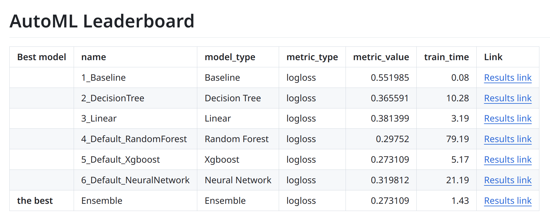
10. AutoML (Automated Machine Learning)

AutoML automates the process of model selection, hyperparameter tuning, and often data preprocessing as well. This saves a lot of time because you do not have to try many algorithms manually. You can just let the AutoML tool explore different pipelines, and it usually returns a high-quality model with less effort on your part.

Back in 2016 I started to work on AutoML to simplify the process of machine learning pipeline learning. I create open-source AutoML system MLJAR Supervised it is available on GitHub at https://github.com/mljar/mljar-supervised.

How It Works

1. An AutoML system combines different algorithms to find the best machine learning pipeline for your dataset.
2. It might automatically perform data cleaning, feature engineering, model selection, hyperparameter tuning, and even create ensembles.
3. While AutoML can be time-consuming for large datasets (since it tries many configurations), it often leads to excellent predictive performance with minimal human intervention.

Example Use Case

Suppose you have a dataset for a new problem and do not know which model will work best—Random Forest, XGBoost, LightGBM, or a neural network. An AutoML system can run all of these, tune them automatically, and then combine the best ones. It will produce a pipeline that you can deploy without needing a deep understanding of each algorithm.

References

• Feurer, M., Klein, A., Eggensperger, K., Springenberg, J., Blum, M., & Hutter, F. (2015). Efficient and robust automated machine learning. In Advances in Neural Information Processing Systems (pp. 2962–2970).

Conclusion

These ten algorithms each have unique strengths:

1. K-Nearest Neighbors (KNN) – Extremely intuitive, no complex training phase, and easy to implement.
2. Decision Trees – Fast training and easy interpretation through a tree structure.
3. Random Forest – Improves performance by combining multiple trees, plus provides feature importance.
4. XGBoost – Very fast, handles missing data well, and continues to dominate many Kaggle competitions.
5. LightGBM – Efficient, flexible gradient boosting with a clever leaf-wise growth strategy.
6. Multi-Layer Perceptron (MLP) – Simple neural network architecture that can handle many small- to medium-scale tasks.
7. Ensemble Methods – Powerful combination of different models to boost overall accuracy.
8. Genetic Algorithm – Mimics natural selection and can be used for creative feature engineering or parameter optimization.
9. Random Search – Quick, effective, and surprisingly good for finding decent hyperparameters.
10. AutoML – Automates model selection, hyperparameter tuning, and pipeline building, saving a lot of time.

In practice, no single algorithm is always the best. Different problems call for different solutions, and sometimes you will see the best results by mixing techniques or by using AutoML to do the work for you. The algorithms listed above, however, form a strong base for tackling most supervised learning tasks—both classification and regression. If you keep these methods in mind, you will have a robust toolkit for exploring and solving a variety of Machine Learning challenges.

References

1. Cover, T. & Hart, P. (1967). Nearest neighbor pattern classification. IEEE Transactions on Information Theory, 13(1), 21–27.
2. Quinlan, J. R. (1986). Induction of decision trees. Machine Learning, 1(1), 81–106.
3. Breiman, L. (2001). Random forests. Machine Learning, 45(1), 5–32.
4. Chen, T. & Guestrin, C. (2016). XGBoost: A scalable tree boosting system. In Proceedings of the 22nd ACM SIGKDD International Conference on Knowledge Discovery and Data Mining (pp. 785–794).
5. Ke, G., Meng, Q., Finley, T., Wang, T., Chen, W., Ma, W., Ye, Q., & Liu, T.-Y. (2017). LightGBM: A highly efficient gradient boosting decision tree. In Advances in Neural Information Processing Systems (pp. 3149–3157).
6. Rumelhart, D. E., Hinton, G. E., & Williams, R. J. (1986). Learning representations by back-propagating errors. Nature, 323(6088), 533–536.
7. Wolpert, D. H. (1992). Stacked generalization. Neural Networks, 5(2), 241–259.
8. Breiman, L. (1996). Bagging predictors. Machine Learning, 24(2), 123–140.
9. Holland, J. H. (1975). Adaptation in natural and artificial systems. University of Michigan Press.
10. Bergstra, J. & Bengio, Y. (2012). Random search for hyper-parameter optimization. Journal of Machine Learning Research, 13, 281–305.
11. Feurer, M., Klein, A., Eggensperger, K., Springenberg, J., Blum, M., & Hutter, F. (2015). Efficient and robust automated machine learning. In Advances in Neural Information Processing Systems (pp. 2962–2970).