AutoML Technological Use Case
How AutoML Can Help
We're going to use a credit card fraud detection dataset in this instance. Its purpose is to forecast the probability of a fraudulent transaction. 284,807 data samples of transactions total in this extensive dataset. These samples comprise a range of attributes, including transaction amount, duration, and anonymised features obtained by principal component analysis (PCA). Our goal is to create prediction models that correctly identify fraudulent transactions by studying this information. This will assist financial institutions reduce losses and safeguard customers from fraud. Financial institutions' approaches to fraud detection, risk management, and data analysis are being completely transformed by AutoML. MLJAR AutoML provides many advantages through model development process automation that result in notable business growth.
Business Value
30%
Faster
When compared to conventional approaches, MLJAR AutoML can shorten the time needed for model development by about 30%, which might encourage creativity and shorten the time it takes for new features and products to reach the market.
25%
More Scalable
By improving scalability and flexibility by approximately 25%, MLJAR AutoML tools facilitate the handling of various data sources and enable adaptation to evolving business requirements and technology breakthroughs.
40%
More Accessible
MLJAR AutoML systems have the potential to democratize AI capabilities by making advanced machine learning techniques 40% more approachable for teams lacking deep knowledge. This will enable more teams to include machine learning into their projects.
20%
More Competitive
Tech companies can get a 20% competitive advantage by using MLJAR AutoML, which speeds up the construction and deployment of sophisticated machine learning models and improves product differentiation and market positioning.
AutoML Report
MLJAR AutoML offers profound insights into model performance, data analysis, and assessment metrics through its capacity to provide extensive reports filled with insightful data. Here are a couple such examples.
Leaderboard
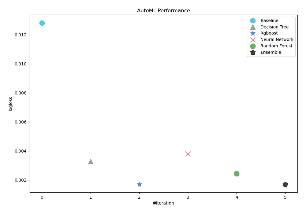
To evaluate the effectiveness of trained models, AutoML has used logloss as its performance measure. As can be seen in the table and graph below, 3_Default_Xgboost was consequently chosen as the best model.
| Best model | name | model_type | metric_type | metric_value | train_time |
|---|---|---|---|---|---|
| 1_Baseline | Baseline | logloss | 0.0128227 | 1.96 | |
| 2_DecisionTree | Decision Tree | logloss | 0.00327765 | 27.18 | |
| the best | 3_Default_Xgboost | Xgboost | logloss | 0.00171326 | 17.88 |
| 4_Default_NeuralNetwork | Neural Network | logloss | 0.00380802 | 28.83 | |
| 5_Default_RandomForest | Random Forest | logloss | 0.00244796 | 38.73 | |
| Ensemble | Ensemble | logloss | 0.00171326 | 6.43 |
AutoML Performance
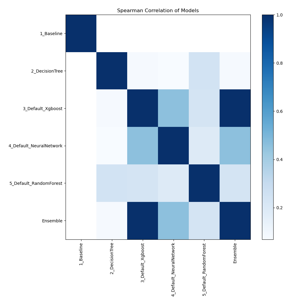
Spearman Correlation of Models
The plot illustrates the relationships between different models based on their rank-order correlation. Spearman correlation measures how well the relationship between two variables can be described using a monotonic function, highlighting the strength of the models' performance rankings. Higher correlation values indicate stronger relationships, where models perform similarly across different metrics or datasets.
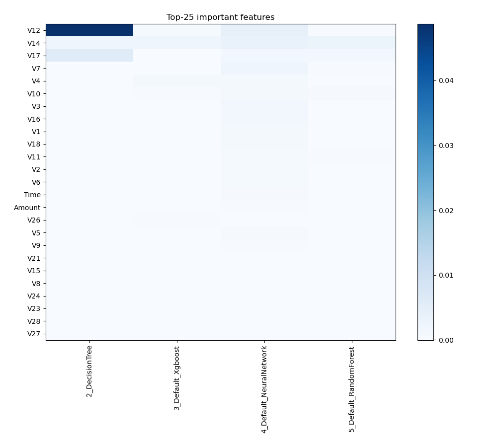
Feature Importance
The plot visualizes the significance of various features across different models. In this heatmap, each cell represents the importance of a specific feature for a particular model, with the color intensity indicating the level of importance. Darker or more intense colors signify higher importance, while lighter colors indicate lower importance. This visualization helps in comparing the contribution of features across multiple models, highlighting which features consistently play a critical role and which are less influential in predictive performance.
Install and import necessary packages
Install the packages with the command:
pip install pandas, mljar-supervised, scikit-learn
Import the packages into your code:
# import packages
import pandas as pd
from supervised import AutoML
from sklearn.model_selection import train_test_split
from sklearn.metrics import accuracy_score
Load data
Import the dataset containing information about credit card fraud.
# read data from csv file
df = pd.read_csv(r"C:\Users\Your_user\technological-use-case\creditcard.csv")
# display data shape
print(f"Loaded data shape {df.shape}")
# display first rows
df.head()
Loaded data shape (284807, 31)
| Time | V1 | V2 | V3 | V4 | V5 | V6 | V7 | V8 | V9 | ... | V21 | V22 | V23 | V24 | V25 | V26 | V27 | V28 | Amount | Class | |
|---|---|---|---|---|---|---|---|---|---|---|---|---|---|---|---|---|---|---|---|---|---|
| 0 | 0.0 | -1.359807 | -0.072781 | 2.536347 | 1.378155 | -0.338321 | 0.462388 | 0.239599 | 0.098698 | 0.363787 | ... | -0.018307 | 0.277838 | -0.110474 | 0.066928 | 0.128539 | -0.189115 | 0.133558 | -0.021053 | 149.62 | 0 |
| 1 | 0.0 | 1.191857 | 0.266151 | 0.166480 | 0.448154 | 0.060018 | -0.082361 | -0.078803 | 0.085102 | -0.255425 | ... | -0.225775 | -0.638672 | 0.101288 | -0.339846 | 0.167170 | 0.125895 | -0.008983 | 0.014724 | 2.69 | 0 |
| 2 | 1.0 | -1.358354 | -1.340163 | 1.773209 | 0.379780 | -0.503198 | 1.800499 | 0.791461 | 0.247676 | -1.514654 | ... | 0.247998 | 0.771679 | 0.909412 | -0.689281 | -0.327642 | -0.139097 | -0.055353 | -0.059752 | 378.66 | 0 |
| 3 | 1.0 | -0.966272 | -0.185226 | 1.792993 | -0.863291 | -0.010309 | 1.247203 | 0.237609 | 0.377436 | -1.387024 | ... | -0.108300 | 0.005274 | -0.190321 | -1.175575 | 0.647376 | -0.221929 | 0.062723 | 0.061458 | 123.50 | 0 |
| 4 | 2.0 | -1.158233 | 0.877737 | 1.548718 | 0.403034 | -0.407193 | 0.095921 | 0.592941 | -0.270533 | 0.817739 | ... | -0.009431 | 0.798278 | -0.137458 | 0.141267 | -0.206010 | 0.502292 | 0.219422 | 0.215153 | 69.99 | 0 |
5 rows × 31 columns
Split dataframe to train/test
To split a dataframe into train and test sets, we divide the data to create separate datasets for training and evaluating a model. This ensures we can assess the model's performance on unseen data.
This step is essential when you have only one base dataset.
# split data
train, test = train_test_split(df, train_size=0.95, shuffle=True, random_state=42)
# display data shapes
print(f"All data shape {df.shape}")
print(f"Train shape {train.shape}")
print(f"Test shape {test.shape}")
All data shape (284807, 31)
Train shape (270566, 31)
Test shape (14241, 31)
Select X,y for ML training
We will split the training set into features (X) and target (y) variables for model training.
# create X columns list and set y column
x_cols = ["Time", "V1", "V2", "V3", "V4", "V5", "V6", "V7", "V8", "V9", "V10", "V11", "V12", "V13", "V14", "V15", "V16", "V17", "V18", "V19", "V20", "V21", "V22", "V23", "V24", "V25", "V26", "V27", "V28", "Amount"]
y_col = "Class"
# set input matrix
X = train[x_cols]
# set target vector
y = train[y_col]
# display data shapes
print(f"X shape is {X.shape}")
print(f"y shape is {y.shape}")
X shape is (270566, 30)
y shape is (270566,)
Fit AutoML
We need to train a model for our dataset. The fit() method will handle the model training and optimization automatically.
# create automl object
automl = AutoML(total_time_limit=300, mode="Explain")
# train automl
automl.fit(X, y)
Compute predictions
Use the trained AutoML model to make predictions on test data.
# predict with AutoML
predictions = automl.predict(test)
# predicted values
print(predictions)
[1 0 0 ... 0 0 0]
Compute accuracy
We need to retrieve the true values of credit card fraud to compare with our predictions. After that, we compute the accuracy score.
# get true values of fraud
true_values = test["Class"]
# compute metric
metric_accuracy = accuracy_score(true_values, predictions)
print(f"Accuracy: {metric_accuracy}")
Accuracy: 0.9915736254476512
Conlusions
When applied to climate model simulations, MLJAR AutoML provides a number of benefits for enhancing model dependability and comprehending accidents in the simulation. MLJAR AutoML improves the precision of simulation results prediction and failure root cause analysis by automating the intricate process of data analysis. Due to this advanced automation, researchers can handle large amounts of simulation data quickly and effectively, identifying trends and other elements that they might have missed using more conventional techniques. The increasing assimilation of this technology has potential to propel our comprehension of climate processes and augment the accuracy of climate forecasts.
See you soon👋.