AutoML Mobile Price Use Case
How AutoML Can Help
The Mobile Price dataset contains a variety of mobile phone-related characteristics, such as RAM, internal storage, screen size, and CPU type, which are used to forecast the price range of these devices. This dataset offers a thorough understanding of how various specifications affect the cost of mobile phones, providing valuable information to makers and users alike. In this situation, MLJAR AutoML can greatly improve the process of mobile price prediction. MLJAR AutoML simplifies the process of developing predictive models by automating the processes of model selection, tuning, and evaluation. This guarantees precise and effective forecasts of mobile phone costs. In the end, this automation helps stakeholders make intelligent choices about mobile device pricing strategies and market positioning by not only simplifying the model generation process but also aiding in the identification of key factors that impact pricing.
Business Value
25%
More Accurate
When compared to previous methods, AutoML can increase pricing prediction accuracy by up to 25%, resulting in more accurate pricing strategies that better reflect customer demand and market realities.
30%
Cost Reduction
By automating the model-building process, MLJAR AutoML can decrease the costs associated with data science and model development by approximately 30%, freeing up resources for other strategic initiatives.
40%
Accelerated Model Development
MLJAR AutoML can reduce the time required to develop and deploy predictive models for mobile prices by up to 40%, allowing businesses to quickly adapt to market changes and optimize pricing strategies.
AutoML Report
MLJAR AutoML offers profound insights into model performance, data analysis, and assessment metrics through its capacity to provide extensive reports filled with insightful data. Here are a couple such examples.
Leaderboard
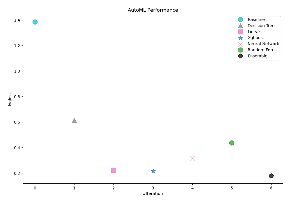
To evaluate the effectiveness of trained models, AutoML has used logloss as its performance measure. As can be seen in the table and graph below, Ensemble was consequently chosen as the best model.
| Best model | name | model_type | metric_type | metric_value | train_time |
|---|---|---|---|---|---|
| 1_Baseline | Baseline | logloss | 1.38629 | 0.56 | |
| 2_DecisionTree | Decision Tree | logloss | 0.614034 | 14.36 | |
| 3_Linear | Linear | logloss | 0.222379 | 7.27 | |
| 4_Default_Xgboost | Xgboost | logloss | 0.216422 | 9.33 | |
| 5_Default_NeuralNetwork | Neural Network | logloss | 0.31977 | 1.1 | |
| 6_Default_RandomForest | Random Forest | logloss | 0.437807 | 7.86 | |
| the best | Ensemble | Ensemble | logloss | 0.180543 | 0.24 |
AutoML Performance
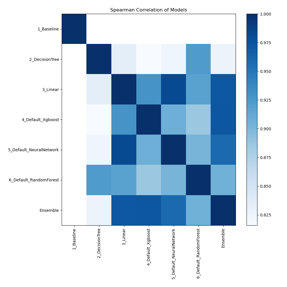
Spearman Correlation of Models
The pairwise Spearman correlation coefficients between various models are shown in the heatmap. The monotonic relationship between the predictions of two models is represented by the strength of each cell. Strong correlations are shown by values around 1 and weak or nonexistent correlations by values near 0. This heatmap allows comprehension of the relative performance of several models in terms of ranking data points.
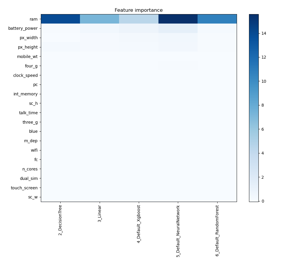
Feature Importance
The plot visualizes the significance of various features across different models. In this heatmap, each cell represents the importance of a specific feature for a particular model, with the color intensity indicating the level of importance. Darker or more intense colors signify higher importance, while lighter colors indicate lower importance. This visualization helps in comparing the contribution of features across multiple models, highlighting which features consistently play a critical role and which are less influential in predictive performance.
Install and import necessary packages
Install the packages with the command:
pip install pandas, mljar-supervised
Import the packages into your code:
# import packages
import pandas as pd
from supervised import AutoML
Load training data
Import the dataset containing information about mobile prices.
# read data from csv file
train = pd.read_csv(r"C:\Users\my_notebooks\train.csv")
# display data shape
print(train.shape)
# display first rows
train.head()
(2000, 21)
| battery_power | blue | clock_speed | dual_sim | fc | four_g | int_memory | m_dep | mobile_wt | n_cores | ... | px_height | px_width | ram | sc_h | sc_w | talk_time | three_g | touch_screen | wifi | price_range | |
|---|---|---|---|---|---|---|---|---|---|---|---|---|---|---|---|---|---|---|---|---|---|
| 0 | 842 | 0 | 2.2 | 0 | 1 | 0 | 7 | 0.6 | 188 | 2 | ... | 20 | 756 | 2549 | 9 | 7 | 19 | 0 | 0 | 1 | 1 |
| 1 | 1021 | 1 | 0.5 | 1 | 0 | 1 | 53 | 0.7 | 136 | 3 | ... | 905 | 1988 | 2631 | 17 | 3 | 7 | 1 | 1 | 0 | 2 |
| 2 | 563 | 1 | 0.5 | 1 | 2 | 1 | 41 | 0.9 | 145 | 5 | ... | 1263 | 1716 | 2603 | 11 | 2 | 9 | 1 | 1 | 0 | 2 |
| 3 | 615 | 1 | 2.5 | 0 | 0 | 0 | 10 | 0.8 | 131 | 6 | ... | 1216 | 1786 | 2769 | 16 | 8 | 11 | 1 | 0 | 0 | 2 |
| 4 | 1821 | 1 | 1.2 | 0 | 13 | 1 | 44 | 0.6 | 141 | 2 | ... | 1208 | 1212 | 1411 | 8 | 2 | 15 | 1 | 1 | 0 | 1 |
5 rows × 21 columns
Select X,y for ML training
We will split the training set into features (X_train) and target (y_train) variables for model training.
# create X columns list and set y column
x_cols = ["battery_power", "blue", "clock_speed", "dual_sim", "fc", "four_g", "int_memory", "m_dep", "mobile_wt", "n_cores", "pc", "px_height", "px_width", "ram", "sc_h", "sc_w", "talk_time", "three_g", "touch_screen", "wifi"]
y_col = "price_range"
# set input matrix
X_train = train[x_cols]
# set target vector
y_train = train[y_col]
# display data shapes
print(f"X_train shape is {X_train.shape}")
print(f"y_train shape is {y_train.shape}")
X_train shape is (2000, 20)
y_train shape is (2000,)
Fit AutoML
We need to train a model for our dataset. The fit() method will handle the model training and optimization automatically.
# create automl object
automl = AutoML(total_time_limit=300, mode="Explain")
# train automl
automl.fit(X_train, y_train)
Load test data
Import the dataset on which we will make predictions.
# read data from csv file
test = pd.read_csv(r"C:\Users\my_notebooks\test.csv")
# display data shape
print(test.shape)
# display first rows
test.head()
(1000, 21)
| id | battery_power | blue | clock_speed | dual_sim | fc | four_g | int_memory | m_dep | mobile_wt | ... | pc | px_height | px_width | ram | sc_h | sc_w | talk_time | three_g | touch_screen | wifi | |
|---|---|---|---|---|---|---|---|---|---|---|---|---|---|---|---|---|---|---|---|---|---|
| 0 | 1 | 1043 | 1 | 1.8 | 1 | 14 | 0 | 5 | 0.1 | 193 | ... | 16 | 226 | 1412 | 3476 | 12 | 7 | 2 | 0 | 1 | 0 |
| 1 | 2 | 841 | 1 | 0.5 | 1 | 4 | 1 | 61 | 0.8 | 191 | ... | 12 | 746 | 857 | 3895 | 6 | 0 | 7 | 1 | 0 | 0 |
| 2 | 3 | 1807 | 1 | 2.8 | 0 | 1 | 0 | 27 | 0.9 | 186 | ... | 4 | 1270 | 1366 | 2396 | 17 | 10 | 10 | 0 | 1 | 1 |
| 3 | 4 | 1546 | 0 | 0.5 | 1 | 18 | 1 | 25 | 0.5 | 96 | ... | 20 | 295 | 1752 | 3893 | 10 | 0 | 7 | 1 | 1 | 0 |
| 4 | 5 | 1434 | 0 | 1.4 | 0 | 11 | 1 | 49 | 0.5 | 108 | ... | 18 | 749 | 810 | 1773 | 15 | 8 | 7 | 1 | 0 | 1 |
5 rows × 21 columns
Compute predictions
Use the trained AutoML model to make predictions of mobile phones prices.
# predict with AutoML
predictions = automl.predict(test)
# predicted values
print(predictions)
[3 3 2 3 1 3 3 1 3 0 3 3 0 0 2 0 2 1 3 2 1 3 1 1 3 0 2 0 2 0 2 0 3 0 1 1 3
 1 2 1 1 2 0 0 0 1 0 3 1 2 1 0 3 0 3 1 3 1 1 3 3 2 0 1 1 1 2 3 1 2 1 2 2 3
 ...
 2 1 1 2 2 3 3 0 2 1 2 1 3 1 1 3 0 2 0 0 3 3 2 0 0 0 0 3 2 3 3 0 0 2 1 0 ]
Display result
We want to see clearly which mobile phone (id) has what price range (Cost).
# create mapping dict
pred_mapping = {0: 'low cost', 1: 'medium cost', 2: 'high cost', 3: 'very high cost'}
# convert list using comprehension
cat_list = [pred_mapping[x] for x in predictions]
# create data frame and display it
result = pd.DataFrame(data = {"Cost": cat_list}, index=test["id"])
result
| id | Cost |
|---|---|
| 1 | very high cost |
| 2 | very high cost |
| 3 | high cost |
| 4 | very high cost |
| 5 | medium cost |
| ... | ... |
| 996 | high cost |
| 997 | medium cost |
| 998 | low cost |
| 999 | high cost |
| 1000 | high cost |
1000 rows × 1 columns
Conlusions
MLJAR AutoML provides significant advantages for pricing strategy optimization and market responsiveness in the mobile price use case. MLJAR AutoML increases price prediction accuracy and facilitates strategic decision-making by automating the complex process of evaluating massive datasets relevant to mobile pricing. Businesses can quickly adjust to market dynamics and customer trends thanks to this automation, which also expedites model development and lowers related expenses. As a result, businesses may implement more accurate pricing plans and maintain their competitiveness in a market that is changing quickly. Pricing strategies could be completely changed by the increasing use of MLJAR AutoML, which offers a competitive advantage through improved productivity and data-driven insights.
See you soon👋.