AutoML Medical Use Case
How AutoML Can Help
MLJAR AutoML simplifies complex medical analysis by automating machine learning processes. It excels in tasks such as diagnosing diseases, predicting patient outcomes, and personalizing treatment plans with remarkable precision and ease. A prime example is the breast cancer dataset, a critical resource in oncology that includes various attributes of tumors to aid in diagnosis. The breast cancer dataset typically features attributes such as tumor size, texture, shape, and other characteristics like smoothness, compactness, and symmetry. By leveraging this dataset, MLJAR AutoML can automate the process of training and validating models that predict tumor malignancy. It employs sophisticated algorithms to analyze patterns and relationships within the data, enhancing diagnostic accuracy. Moreover, MLJAR AutoML’s ability to handle and interpret complex datasets facilitates the development of personalized treatment plans. It enables more accurate risk assessments, which can lead to better-targeted therapies and improved patient outcomes. In summary, the breast cancer dataset is a fundamental component of MLJAR AutoML’s capabilities, driving advancements in medical diagnostics and contributing to more effective healthcare solutions.
Business Value
25%
Better Accuracy
By automating and improving feature selection and model training, MLJAR AutoML can improve diagnostic accuracy by up to 25% for cancer detection and other early diagnoses.
30%
More Effective
MLJAR AutoML can more precisely personalize treatment regimens by evaluating large volumes of patient data, which may boost intervention effectiveness by approximately 30%.
40%
More Efficient
By automating common data analysis and diagnostic procedures, MLJAR AutoML can streamline processes and cut the manual work for medical practitioners by about 40%.
20%
More Optimal
By applying MLJAR AutoML to power predictive models, medical staff and resource allocation can be optimized, potentially leading to a 20% increase in hospital efficiency and resource management.
AutoML Report
MLJAR AutoML produces an extensive report rich with information, delivering valuable insights into model performance, data analysis, and evaluation metrics. Below are some examples.
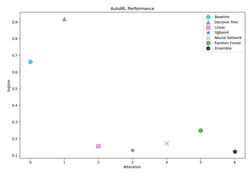
Leaderboard
As logloss was used as a criterion to evaluate trained models' performance, AutoML determined that Ensemble was the best model. The table and graph below display the results.
| Best model | name | model_type | metric_type | metric_value | train_time |
|---|---|---|---|---|---|
| 1_Baseline | Baseline | logloss | 0.660997 | 2.01 | |
| 2_DecisionTree | Decision Tree | logloss | 0.919681 | 20.63 | |
| 3_Linear | Linear | logloss | 0.155132 | 9.58 | |
| 4_Default_Xgboost | Xgboost | logloss | 0.129083 | 13.58 | |
| 5_Default_NeuralNetwork | Neural Network | logloss | 0.171555 | 5.29 | |
| 6_Default_RandomForest | Random Forest | logloss | 0.248971 | 12.84 | |
| the best | Ensemble | Ensemble | logloss | 0.122313 | 3.08 |
Performance
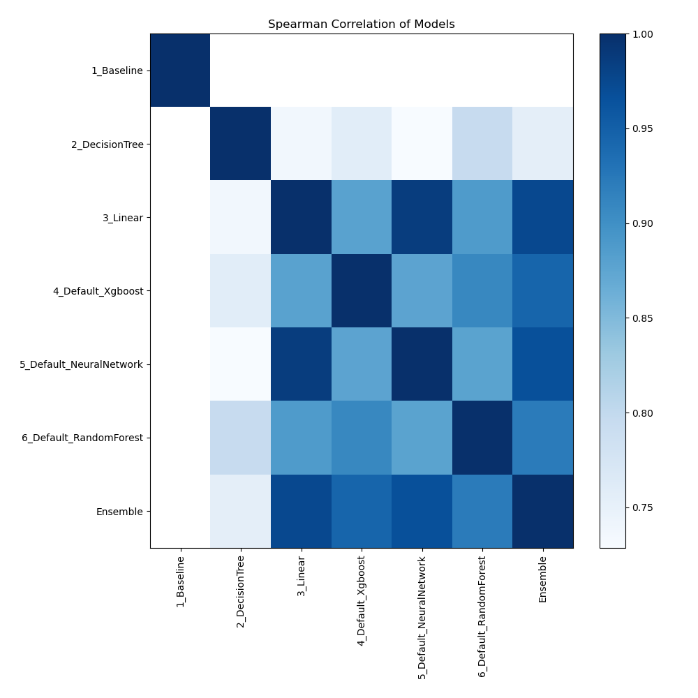
Spearman Correlation of Models
The heatmap provides a visual representation of the pairwise Spearman correlation coefficients between different models. Each cell indicates the strength and direction of the monotonic relationship between the predictions of two models. A value close to 1 indicates a strong correlation, while a value close to 0 indicates a weak or no correlation. This heatmap helps to understand how similarly different models perform in ranking data points.
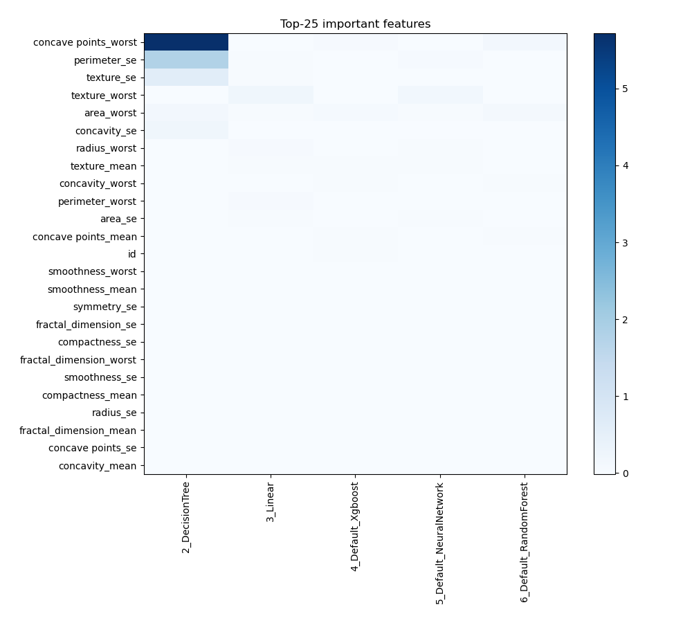
Feature Importance
The graph shows the importance of different features in influencing the model's predictions. Each feature is ranked according to its contribution to the predictive power of the model, with higher values indicating greater importance. This visualization helps to understand which features have the greatest impact on model performance, guiding feature selection and model interpretation efforts.
Install and import necessary packages
Install the packages with the command:
pip install pandas, scikit-learn, mljar-supervised
Import the packages into your code:
# import packages
import pandas as pd
from sklearn.model_selection import train_test_split
from supervised import AutoML
from sklearn.metrics import accuracy_score
Load data
Import the breast cancer dataset for analysis and model building.
# load example dataset
df = pd.read_csv("https://raw.githubusercontent.com/pplonski/datasets-for-start/master/breast_cancer_wisconsin/data.csv")
# display DataFrame shape
print(f"Loaded data shape {df.shape}")
# display first rows
df.head()
Loaded data shape (569, 32)
| id | diagnosis | radius_mean | texture_mean | perimeter_mean | area_mean | smoothness_mean | compactness_mean | concavity_mean | concave points_mean | ... | radius_worst | texture_worst | perimeter_worst | area_worst | smoothness_worst | compactness_worst | concavity_worst | concave points_worst | symmetry_worst | fractal_dimension_worst | |
|---|---|---|---|---|---|---|---|---|---|---|---|---|---|---|---|---|---|---|---|---|---|
| 0 | 842302 | M | 17.99 | 10.38 | 122.80 | 1001.0 | 0.11840 | 0.27760 | 0.3001 | 0.14710 | ... | 25.38 | 17.33 | 184.60 | 2019.0 | 0.1622 | 0.6656 | 0.7119 | 0.2654 | 0.4601 | 0.11890 |
| 1 | 842517 | M | 20.57 | 17.77 | 132.90 | 1326.0 | 0.08474 | 0.07864 | 0.0869 | 0.07017 | ... | 24.99 | 23.41 | 158.80 | 1956.0 | 0.1238 | 0.1866 | 0.2416 | 0.1860 | 0.2750 | 0.08902 |
| 2 | 84300903 | M | 19.69 | 21.25 | 130.00 | 1203.0 | 0.10960 | 0.15990 | 0.1974 | 0.12790 | ... | 23.57 | 25.53 | 152.50 | 1709.0 | 0.1444 | 0.4245 | 0.4504 | 0.2430 | 0.3613 | 0.08758 |
| 3 | 84348301 | M | 11.42 | 20.38 | 77.58 | 386.1 | 0.14250 | 0.28390 | 0.2414 | 0.10520 | ... | 14.91 | 26.50 | 98.87 | 567.7 | 0.2098 | 0.8663 | 0.6869 | 0.2575 | 0.6638 | 0.17300 |
| 4 | 84358402 | M | 20.29 | 14.34 | 135.10 | 1297.0 | 0.10030 | 0.13280 | 0.1980 | 0.10430 | ... | 22.54 | 16.67 | 152.20 | 1575.0 | 0.1374 | 0.2050 | 0.4000 | 0.1625 | 0.2364 | 0.07678 |
5 rows × 32 columns
Split dataframe to train/test
To split a dataframe into train and test sets, we divide the data to create separate datasets for training and evaluating a model. This ensures we can assess the model's performance on unseen data.
This step is essential when you have only one base dataset.
# split data
train, test = train_test_split(df, train_size=0.75, shuffle=True, random_state=42)
# display data shapes
print(f"All data shape {df.shape}")
print(f"Train shape {train.shape}")
print(f"Test shape {test.shape}")
All data shape (569, 32)
Train shape (426, 32)
Test shape (143, 32)
Select X,y for ML training
We will split the training set into features (X_train) and target (y_train) variables for model training.
# create X columns list and set y column
x_cols = ["id", "radius_mean", "texture_mean", "perimeter_mean", "area_mean", "smoothness_mean", "compactness_mean", "concavity_mean", "concave points_mean", "symmetry_mean", "fractal_dimension_mean", "radius_se", "texture_se", "perimeter_se", "area_se", "smoothness_se", "compactness_se", "concavity_se", "concave points_se", "symmetry_se", "fractal_dimension_se", "radius_worst", "texture_worst", "perimeter_worst", "area_worst", "smoothness_worst", "compactness_worst", "concavity_worst", "concave points_worst", "symmetry_worst", "fractal_dimension_worst"]
y_col = "diagnosis"
# set input matrix
X_train = train[x_cols]
# set target vector
y_train = train[y_col]
# display data shapes
print(f"X_train shape is {X_train.shape}")
print(f"y_train shape is {y_train.shape}")
X_train shape is (426, 31)
y_train shape is (426,)
Fit AutoML
We need to train a model for our dataset. The fit() method will handle the model training and optimization automatically.
# create automl object
automl = AutoML(total_time_limit=300, mode="Explain")
# train automl
automl.fit(X_train, y_train)
Compute predictions
Use the trained AutoML model to make predictions on test data to identify cancer cases.
# predict with AutoML
predictions = automl.predict(test)
# predicted values
print(predictions)
['B' 'M' 'M' 'B' 'B' 'M' 'M' 'M' 'B' 'B' 'B' 'M' 'B' 'M' 'B' 'M' 'B' 'B'
 'B' 'M' 'B' 'B' 'M' 'B' 'B' 'B' 'B' 'B' 'B' 'M' 'B' 'B' 'B' 'B' 'B' 'B'
 'M' 'B' 'M' 'B' 'B' 'M' 'B' 'B' 'B' 'B' 'B' 'B' 'B' 'B' 'M' 'M' 'B' 'B'
 'B' 'B' 'B' 'M' 'M' 'B' 'B' 'M' 'M' 'B' 'B' 'B' 'M' 'M' 'B' 'B' 'M' 'M'
 'B' 'M' 'B' 'B' 'B' 'B' 'B' 'B' 'M' 'B' 'B' 'M' 'M' 'M' 'M' 'M' 'B' 'B'
 'B' 'B' 'B' 'B' 'B' 'B' 'M' 'M' 'B' 'M' 'M' 'B' 'M' 'M' 'B' 'B' 'B' 'M'
 'B' 'B' 'M' 'B' 'B' 'M' 'B' 'M' 'B' 'B' 'B' 'M' 'B' 'B' 'B' 'M' 'B' 'M'
 'M' 'B' 'B' 'M' 'M' 'M' 'B' 'B' 'B' 'M' 'B' 'B' 'B' 'M' 'B' 'M' 'B']
Display result
We want to see clearly which patient (id) has what diagnosis (Diagnosis).
# create mapping dict
pred_mapping = {'M': 'malignant', 'B': 'benign'}
# convert list using comprehension
cat_list = [pred_mapping[x] for x in predictions]
# create data frame and display it
result = pd.DataFrame(data = {"Diagnosis": cat_list}, index=test["id"])
result
| id | Diagnosis |
|---|---|
| 87930 | benign |
| 859575 | malignant |
| 8670 | malignant |
| 907915 | benign |
| 921385 | benign |
| ... | ... |
| 861598 | benign |
| 877500 | malignant |
| 905520 | benign |
| 849014 | malignant |
| 90317302 | benign |
143 rows × 1 columns
Compute accuracy
We need to retrieve the true values of employee attrition to compare with our predictions. After that, we compute the accuracy score.
# get true values of diagnosis
true_values = test["diagnosis"]
# compute metric
metric_accuracy = accuracy_score(true_values, predictions)
print(f"Accuracy: {metric_accuracy}")
Accuracy: 0.9790209790209791
Conlusions
The application of MLJAR AutoML in research and diagnosis offers significant advantages. It enables accurate predictions, early detection, and personalized treatment plans by automating complex data analysis. AutoML's ability to handle vast datasets efficiently aids in identifying patterns and insights that might be missed by traditional methods. As this technology progresses, its impact on breast cancer diagnosis and treatment will become increasingly vital, leading to improved patient outcomes and more effective healthcare strategies.
See you soon👋.