AutoML HR Use Case
How AutoML Can Help
In our case, we are using the employee attrition dataset. This dataset includes comprehensive employee information such as age, job role, job satisfaction, monthly income etc. The primary prediction task is to identify which employees are likely to leave the company. With attributes like satisfaction level, work environment, and promotion history, this dataset is ideal for training models to predict employee turnover, which can be applied to various HR strategies such as retention planning and workforce management. MLJAR AutoML is transforming human resources by automating predictive analytics for employee attrition. This advanced tool simplifies the model development process, enabling effective retention strategies, optimizing workforce allocation, and enhancing overall employee satisfaction, all of which contribute to substantial business growth.
Business Value
30%
Faster
The time and effort needed for initial screenings can be greatly decreased using MLJAR AutoML, as it can screen and shortlist resumes approximately 30% faster than with traditional human processes.
40%
More Efficient
Because MLJAR AutoML can handle massive amounts of data 40% more effectively than conventional techniques, HR procedures will continue to be scalable and successful even as the company expands.
25%
More Effective
Compared to traditional methods, MLJAR AutoML can detect employees at danger of leaving 25% more successfully by studying patterns in behavior and feedback.
30%
Less Bias
With thorough data analysis, MLJAR AutoML technologies can eliminate HR decision-making biases by around 30%, producing more equitable and objective results.
AutoML Report
MLJAR AutoML produces an extensive report with plenty of data that throws light on evaluation measures, data analysis, and model performance. Here are a few samples of this.
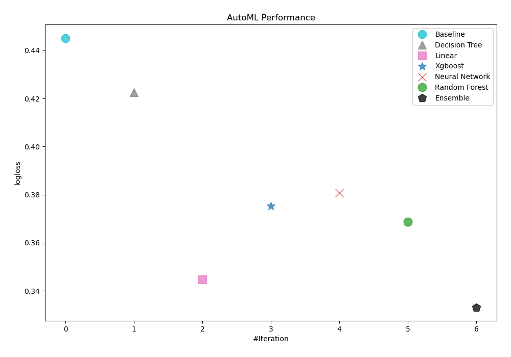
Leaderboard
Logloss is the statistic that AutoML used to evaluate how models performed. The table and graph below show that Ensemble was selected as the best model.
| Best model | name | model_type | metric_type | metric_value | train_time |
|---|---|---|---|---|---|
| 1_Baseline | Baseline | logloss | 0.445174 | 2.16 | |
| 2_DecisionTree | Decision Tree | logloss | 0.422558 | 18.87 | |
| 3_Linear | Linear | logloss | 0.344594 | 9.88 | |
| 4_Default_Xgboost | Xgboost | logloss | 0.375246 | 6.77 | |
| 5_Default_NeuralNetwork | Neural Network | logloss | 0.380813 | 5.42 | |
| 6_Default_RandomForest | Random Forest | logloss | 0.368629 | 11.51 | |
| the best | Ensemble | Ensemble | logloss | 0.333119 | 3.29 |
Performance
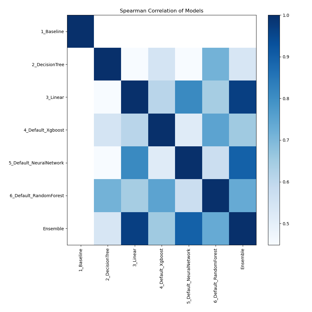
Spearman Correlation of Models
The heatmap shows the pairwise Spearman correlation coefficients between multiple models. The degree and direction of the monotonic relationship between the two models' predictions are shown by each cell. Strong correlations are shown by values near to 1, and weak or no correlations are indicated by values near to 0. This heatmap makes it easier to see how well various models order data points in relation to one another.
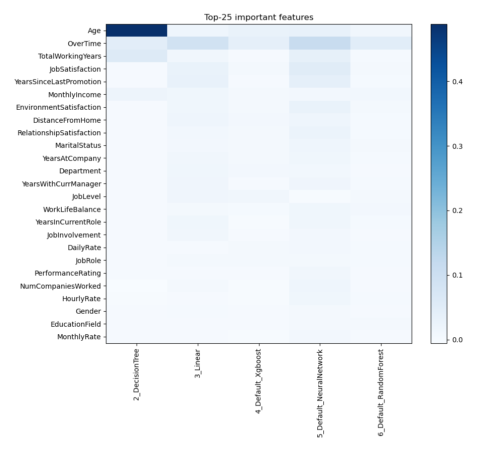
Feature Importance
The graph illustrates how various features affect how the model predicts things. Every characteristic is assigned a value based on how much it adds to the model's predictive power; larger numbers signify more significance. This visualization helps in the understanding of which features most influence the performance of the model, directing efforts related to feature selection and model interpretation.
Install and import necessary packages
Install the packages with the command:
pip install pandas, mljar-supervised, scikit-learn
Import the packages into your code:
# import packages
import pandas as pd
from supervised import AutoML
from sklearn.metrics import accuracy_score
Load training data
Import the employee attrition dataset containing information about employees.
# load example dataset
train = pd.read_csv("https://raw.githubusercontent.com/pplonski/datasets-for-start/master/employee_attrition/HR-Employee-Attrition-train.csv")
# display DataFrame shape
print(f"Loaded data shape {train.shape}")
# display first rows
train.head()
Loaded data shape (1200, 35)
| Age | Attrition | BusinessTravel | DailyRate | Department | DistanceFromHome | Education | EducationField | EmployeeCount | EmployeeNumber | ... | RelationshipSatisfaction | StandardHours | StockOptionLevel | TotalWorkingYears | TrainingTimesLastYear | WorkLifeBalance | YearsAtCompany | YearsInCurrentRole | YearsSinceLastPromotion | YearsWithCurrManager | |
|---|---|---|---|---|---|---|---|---|---|---|---|---|---|---|---|---|---|---|---|---|---|
| 0 | 55 | No | Travel_Rarely | 452 | Research & Development | 1 | 3 | Medical | 1 | 374 | ... | 3 | 80 | 0 | 37 | 2 | 3 | 36 | 10 | 4 | 13 |
| 1 | 47 | Yes | Non-Travel | 666 | Research & Development | 29 | 4 | Life Sciences | 1 | 376 | ... | 4 | 80 | 1 | 10 | 2 | 2 | 10 | 7 | 9 | 9 |
| 2 | 28 | No | Travel_Rarely | 1158 | Research & Development | 9 | 3 | Medical | 1 | 377 | ... | 4 | 80 | 1 | 5 | 3 | 2 | 5 | 2 | 0 | 4 |
| 3 | 37 | No | Travel_Rarely | 228 | Sales | 6 | 4 | Medical | 1 | 378 | ... | 2 | 80 | 1 | 7 | 5 | 4 | 5 | 4 | 0 | 1 |
| 4 | 21 | No | Travel_Rarely | 996 | Research & Development | 3 | 2 | Medical | 1 | 379 | ... | 1 | 80 | 0 | 3 | 4 | 4 | 3 | 2 | 1 | 0 |
5 rows × 35 columns
Select X,y for ML training
Identify the feature variables (X), such as employee attributes, and the target variable (y), such as whether the employee left or stayed.
# create X columns list and set y column
x_cols = ["Age", "BusinessTravel", "DailyRate", "Department", "DistanceFromHome", "Education", "EducationField", "EmployeeCount", "EmployeeNumber", "EnvironmentSatisfaction", "Gender", "HourlyRate", "JobInvolvement", "JobLevel", "JobRole", "JobSatisfaction", "MaritalStatus", "MonthlyIncome", "MonthlyRate", "NumCompaniesWorked", "Over18", "OverTime", "PercentSalaryHike", "PerformanceRating", "RelationshipSatisfaction", "StandardHours", "StockOptionLevel", "TotalWorkingYears", "TrainingTimesLastYear", "WorkLifeBalance", "YearsAtCompany", "YearsInCurrentRole", "YearsSinceLastPromotion", "YearsWithCurrManager"]
y_col = "Attrition"
# set input matrix
X = train[x_cols]
# set target vector
y = train[y_col]
# display data shapes
print(f"X shape is {X.shape}")
print(f"y shape is {y.shape}")
X shape is (1200, 34)
y shape is (1200,)
Fit AutoML
Train the AutoML model using the fit() method to predict employee attrition.
# create automl object
automl = AutoML(total_time_limit=300, mode="Explain")
# train automl
automl.fit(X, y)
Load test data
Let's load test data. We have Target in Attrition column, so we will check accuracy of our predictions later on. We will predict it with AutoML.
# load example dataset
test = pd.read_csv("https://raw.githubusercontent.com/pplonski/datasets-for-start/master/employee_attrition/HR-Employee-Attrition-test.csv")
# display DataFrame shape
print(f"Loaded data shape {test.shape}")
# display first rows
test.head()
Loaded data shape (270, 35)
| Age | Attrition | BusinessTravel | DailyRate | Department | DistanceFromHome | Education | EducationField | EmployeeCount | EmployeeNumber | ... | RelationshipSatisfaction | StandardHours | StockOptionLevel | TotalWorkingYears | TrainingTimesLastYear | WorkLifeBalance | YearsAtCompany | YearsInCurrentRole | YearsSinceLastPromotion | YearsWithCurrManager | |
|---|---|---|---|---|---|---|---|---|---|---|---|---|---|---|---|---|---|---|---|---|---|
| 0 | 41 | Yes | Travel_Rarely | 1102 | Sales | 1 | 2 | Life Sciences | 1 | 1 | ... | 1 | 80 | 0 | 8 | 0 | 1 | 6 | 4 | 0 | 5 |
| 1 | 49 | No | Travel_Frequently | 279 | Research & Development | 8 | 1 | Life Sciences | 1 | 2 | ... | 4 | 80 | 1 | 10 | 3 | 3 | 10 | 7 | 1 | 7 |
| 2 | 37 | Yes | Travel_Rarely | 1373 | Research & Development | 2 | 2 | Other | 1 | 4 | ... | 2 | 80 | 0 | 7 | 3 | 3 | 0 | 0 | 0 | 0 |
| 3 | 33 | No | Travel_Frequently | 1392 | Research & Development | 3 | 4 | Life Sciences | 1 | 5 | ... | 3 | 80 | 0 | 8 | 3 | 3 | 8 | 7 | 3 | 0 |
| 4 | 27 | No | Travel_Rarely | 591 | Research & Development | 2 | 1 | Medical | 1 | 7 | ... | 4 | 80 | 1 | 6 | 3 | 3 | 2 | 2 | 2 | 2 |
5 rows × 35 columns
Compute predictions
Generate predictions on the testing data to identify the likelihood of employee turnover.
# predict with AutoML
predictions = automl.predict(test)
# predicted values
print(predictions)
['Yes' 'No' 'No' 'No' 'No' 'No' 'No' 'No' 'No' 'No' 'No' 'No' 'No' 'No'
 'Yes' 'No' 'No' 'No' 'No' 'No' 'No' 'No' 'No' 'No' 'No' 'No' 'Yes' 'No'
 'No' 'No' 'No' 'No' 'No' 'No' 'Yes' 'No' 'No' 'No' 'Yes' 'No' 'No' 'No'
 'Yes' 'No' 'No' 'No' 'No' 'No' 'No' 'No' 'No' 'Yes' 'No' 'No' 'Yes' 'No'
 'No' 'Yes' 'No' 'No' 'No' 'No' 'No' 'No' 'No' 'No' 'No' 'No' 'No' 'No'
 'No' 'No' 'No' 'No' 'No' 'No' 'No' 'No' 'No' 'No' 'No' 'No' 'No' 'No'
 'No' 'No' 'No' 'No' 'No' 'No' 'No' 'No' 'No' 'No' 'No' 'No' 'No' 'No'
 'No' 'No' 'No' 'No' 'No' 'No' 'No' 'No' 'No' 'No' 'No' 'No' 'No' 'No'
 'No' 'No' 'No' 'No' 'No' 'No' 'No' 'No' 'No' 'No' 'Yes' 'No' 'Yes' 'No'
 'No' 'Yes' 'No' 'No' 'No' 'No' 'Yes' 'No' 'No' 'No' 'No' 'No' 'No' 'No'
 'Yes' 'No' 'No' 'No' 'No' 'No' 'No' 'No' 'No' 'No' 'No' 'No' 'No' 'No'
 'No' 'No' 'No' 'No' 'No' 'No' 'No' 'No' 'No' 'No' 'No' 'No' 'No' 'No'
 'No' 'No' 'No' 'No' 'No' 'No' 'No' 'No' 'No' 'No' 'No' 'No' 'No' 'No'
 'No' 'No' 'No' 'No' 'No' 'No' 'No' 'No' 'No' 'No' 'Yes' 'No' 'No' 'No'
 'No' 'No' 'No' 'No' 'No' 'No' 'No' 'No' 'Yes' 'No' 'No' 'No' 'No' 'No'
 'No' 'No' 'No' 'No' 'No' 'No' 'No' 'No' 'No' 'No' 'No' 'No' 'No' 'No'
 'No' 'No' 'No' 'No' 'No' 'No' 'No' 'No' 'No' 'No' 'No' 'No' 'No' 'No'
 'No' 'No' 'No' 'No' 'No' 'No' 'No' 'No' 'No' 'No' 'No' 'No' 'No' 'No'
 'No' 'No' 'No' 'No' 'No' 'No' 'No' 'No' 'No' 'No' 'No' 'No' 'No' 'No'
 'No' 'No' 'No' 'No']
Display result
We want to see clearly our predictions.
# create data frame and display it
result = pd.DataFrame(data={"Attrition": predictions})
result
| Attrition | |
|---|---|
| 0 | Yes |
| 1 | No |
| 2 | No |
| 3 | No |
| 4 | No |
| ... | ... |
| 265 | No |
| 266 | No |
| 267 | No |
| 268 | No |
| 269 | No |
270 rows × 1 columns
Compute accuracy
We need to retrieve the true values of employee attrition to compare with our predictions. After that, we compute the accuracy score.
# select true value column
true_values = test["Attrition"]
# compute metric
metric_accuracy = accuracy_score(true_values, predictions)
print(f"Accuracy: {metric_accuracy}")
Accuracy: 0.8777777777777778
Conlusions
Using MLJAR AutoML makes predicting employee attrition easier. It automatically builds and fine-tunes models, so HR teams can quickly analyze employee data and spot those likely to leave. With AutoML, there's less need for manual data work, making it a handy tool for improving staff retention.
See you soon👋.