AutoML Housing Use Case
How AutoML Can Help
MLJAR AutoML simplifies complex housing market analysis by automating the application of machine learning models. The tool helps with a variety of housing-related tasks such as predicting property prices, identifying market trends and evaluating investment opportunities with high precision and ease. To present we are going to use the house-prices dataset, which contains 1,460 samples and, as usual, includes various characteristics such as area, number of bedrooms and bathrooms, location, year of construction and others. These features are used to predict house prices by capturing the relationship between property features and market values. MLJAR AutoML drives business growth by automating complex data analysis, enabling precise insights and forecasts that empower companies to make informed decisions and seize market opportunities with confidence.
Business Value
25%
More Accurate Price Predictions
When compared to conventional approaches, MLJAR AutoML improves price predictions by about 25% and offers accurate property value estimates.
20%
Improved Forecasting
Using property data, MLJAR AutoML improves the assessment of possible investments by providing a 20% increase in forecasting accuracy for future price changes.
30%
Better Trend Detection
MLJAR AutoML's sophisticated algorithms enable it to detect new trends and changes in the housing market up to 30% more accurately, which improves strategic maneuvers.
25%
Better Strategic Planning
By utilizing cutting-edge machine learning, MLJAR AutoML can enhance strategic planning and operational efficiency by approximately 25% by optimizing decision-making processes.
AutoML Report
MLJAR AutoML creates a detailed report filled with valuable information, offering deep insights into model performance, data analysis, and evaluation metrics. Here are some examples.
Leaderboard
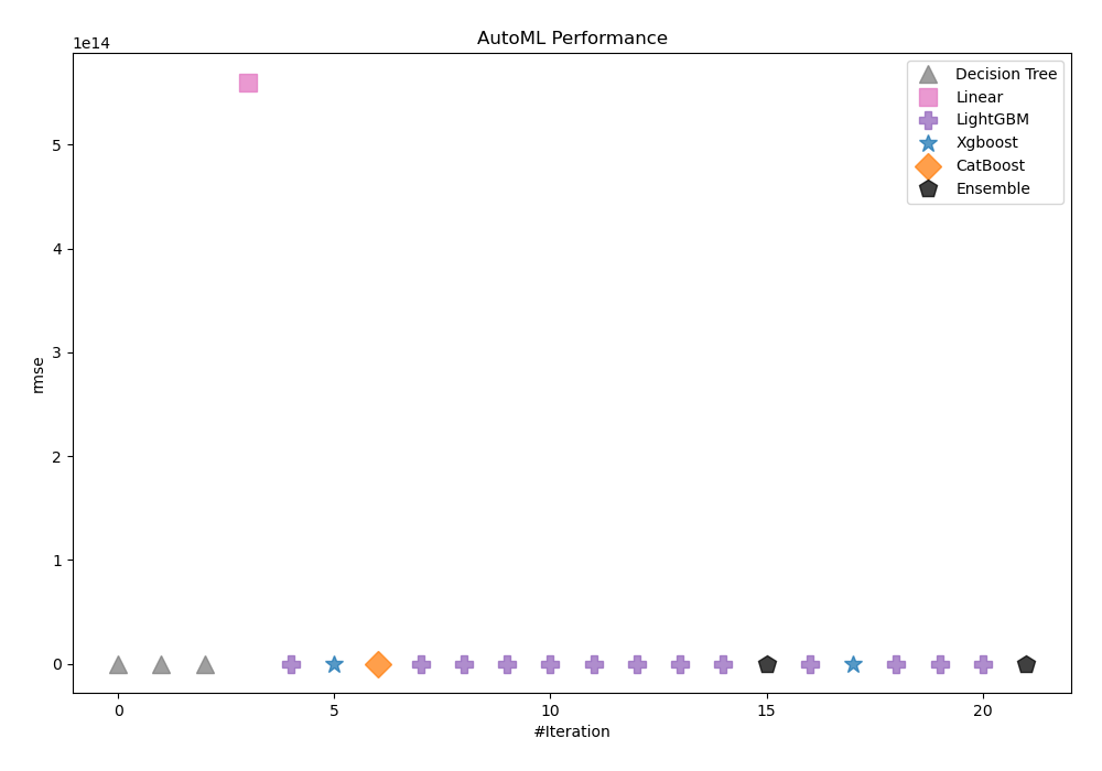
In this case, we used Compete mode to better determine housing prices. It uses feature generation and Stacked Ensemble techniques. AutoML chose rmse as the metric it would use to measure the performance of trained models. It then selected Ensemble_Stacked as the best model, as shown in the table and chart below.
| Best model | name | model_type | metric_type | metric_value | train_time |
|---|---|---|---|---|---|
| 1_DecisionTree | Decision Tree | rmse | 45384.9 | 2.8 | |
| 2_DecisionTree | Decision Tree | rmse | 41576.1 | 2.7 | |
| 3_DecisionTree | Decision Tree | rmse | 41576.1 | 2.75 | |
| 4_Linear | Linear | rmse | 5.60193e+14 | 4.07 | |
| 5_Default_LightGBM | LightGBM | rmse | 28368.7 | 6.02 | |
| 6_Default_Xgboost | Xgboost | rmse | 28406.3 | 8.36 | |
| 7_Default_CatBoost | CatBoost | rmse | 26154.6 | 125.91 | |
| 5_Default_LightGBM_GoldenFeatures | LightGBM | rmse | 28917.3 | 15.85 | |
| 5_Default_LightGBM_KMeansFeatures | LightGBM | rmse | 28909.9 | 6.83 | |
| 5_Default_LightGBM_RandomFeature | LightGBM | rmse | 28918.4 | 12.34 | |
| 5_Default_LightGBM_SelectedFeatures | LightGBM | rmse | 26587.2 | 14.35 | |
| 10_LightGBM_SelectedFeatures | LightGBM | rmse | 27225.5 | 5.03 | |
| 11_LightGBM_SelectedFeatures | LightGBM | rmse | 26835.3 | 28.96 | |
| 14_LightGBM_SelectedFeatures | LightGBM | rmse | 27387.4 | 6.24 | |
| 5_Default_LightGBM_SelectedFeatures_BoostOnErrors | LightGBM | rmse | 27911.5 | 6.12 | |
| Ensemble | Ensemble | rmse | 25373.1 | 0.7 | |
| 5_Default_LightGBM_SelectedFeatures_Stacked | LightGBM | rmse | 26498.7 | 5.83 | |
| 6_Default_Xgboost_Stacked | Xgboost | rmse | 26029.1 | 6.06 | |
| 11_LightGBM_SelectedFeatures_Stacked | LightGBM | rmse | 26557.4 | 6.48 | |
| 10_LightGBM_SelectedFeatures_Stacked | LightGBM | rmse | 26327.8 | 5.22 | |
| 14_LightGBM_SelectedFeatures_Stacked | LightGBM | rmse | 26467.9 | 6.11 | |
| the best | Ensemble_Stacked | Ensemble | rmse | 25030.3 | 1.08 |
Performance
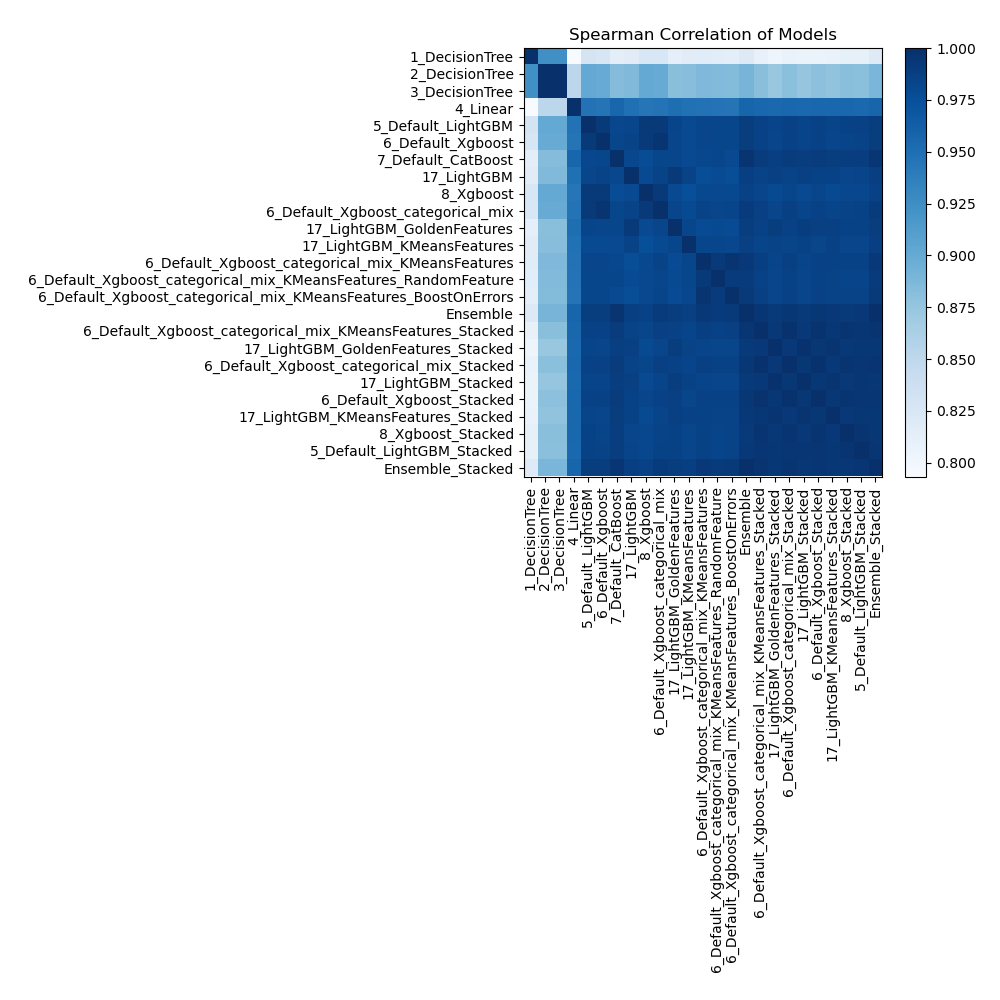
Spearman Correlation of Models
The pairwise Spearman correlation coefficients between various models are shown in the heatmap. The monotonic relationship between the predictions of two models is represented by the strength of each cell. Strong correlations are shown by values around 1 and weak or nonexistent correlations by values near 0. This heatmap allows comprehension of the relative performance of several models in terms of ranking data points.
Install and import necessary packages
Install the packages with the command:
pip install pandas, scikit-learn, mljar-supervised
Import the packages into your code:
# import packages
import pandas as pd
from sklearn.model_selection import train_test_split
from supervised import AutoML
Load data
We will read data from a house-prices dataset.
# load example dataset
df = pd.read_csv("https://raw.githubusercontent.com/pplonski/datasets-for-start/master/house_prices/data.csv")
# display DataFrame shape
print(f"Loaded data shape {df.shape}")
# display first rows
df.head()
Loaded data shape (1460, 81)
| Id | MSSubClass | MSZoning | LotFrontage | LotArea | Street | Alley | LotShape | LandContour | Utilities | ... | PoolArea | PoolQC | Fence | MiscFeature | MiscVal | MoSold | YrSold | SaleType | SaleCondition | SalePrice | |
|---|---|---|---|---|---|---|---|---|---|---|---|---|---|---|---|---|---|---|---|---|---|
| 0 | 1 | 60 | RL | 65.0 | 8450 | Pave | NaN | Reg | Lvl | AllPub | ... | 0 | NaN | NaN | NaN | 0 | 2 | 2008 | WD | Normal | 208500 |
| 1 | 2 | 20 | RL | 80.0 | 9600 | Pave | NaN | Reg | Lvl | AllPub | ... | 0 | NaN | NaN | NaN | 0 | 5 | 2007 | WD | Normal | 181500 |
| 2 | 3 | 60 | RL | 68.0 | 11250 | Pave | NaN | IR1 | Lvl | AllPub | ... | 0 | NaN | NaN | NaN | 0 | 9 | 2008 | WD | Normal | 223500 |
| 3 | 4 | 70 | RL | 60.0 | 9550 | Pave | NaN | IR1 | Lvl | AllPub | ... | 0 | NaN | NaN | NaN | 0 | 2 | 2006 | WD | Abnorml | 140000 |
| 4 | 5 | 60 | RL | 84.0 | 14260 | Pave | NaN | IR1 | Lvl | AllPub | ... | 0 | NaN | NaN | NaN | 0 | 12 | 2008 | WD | Normal | 250000 |
5 rows × 81 columns
Split dataframe to train/test
To split a dataframe into train and test sets, we divide the data to create separate datasets for training and evaluating a model. This ensures we can assess the model's performance on unseen data.
# split data
train, test = train_test_split(df, train_size=0.95, shuffle=True, random_state=42)
# display data shapes
print(f"All data shape {df.shape}")
print(f"Train shape {train.shape}")
print(f"Test shape {test.shape}")
All data shape (1460, 81)
Train shape (1387, 81)
Test shape (73, 81)
Select X,y for ML training
We will split the training set into features (X) and target (y) variables for model training.
# create X columns list and set y column
x_cols = ["Id", "MSSubClass", "MSZoning", "LotFrontage", "LotArea", "Street", "Alley", "LotShape", "LandContour", "Utilities", "LotConfig", "LandSlope", "Neighborhood", "Condition1", "Condition2", "BldgType", "HouseStyle", "OverallQual", "OverallCond", "YearBuilt", "YearRemodAdd", "RoofStyle", "RoofMatl", "Exterior1st", "Exterior2nd", "MasVnrType", "MasVnrArea", "ExterQual", "ExterCond", "Foundation", "BsmtQual", "BsmtCond", "BsmtExposure", "BsmtFinType1", "BsmtFinSF1", "BsmtFinType2", "BsmtFinSF2", "BsmtUnfSF", "TotalBsmtSF", "Heating", "HeatingQC", "CentralAir", "Electrical", "1stFlrSF", "2ndFlrSF", "LowQualFinSF", "GrLivArea", "BsmtFullBath", "BsmtHalfBath", "FullBath", "HalfBath", "BedroomAbvGr", "KitchenAbvGr", "KitchenQual", "TotRmsAbvGrd", "Functional", "Fireplaces", "FireplaceQu", "GarageType", "GarageYrBlt", "GarageFinish", "GarageCars", "GarageArea", "GarageQual", "GarageCond", "PavedDrive", "WoodDeckSF", "OpenPorchSF", "EnclosedPorch", "3SsnPorch", "ScreenPorch", "PoolArea", "PoolQC", "Fence", "MiscFeature", "MiscVal", "MoSold", "YrSold", "SaleType", "SaleCondition"]
y_col = "SalePrice"
# set input matrix
X = train[x_cols]
# set target vector
y = train[y_col]
# display data shapes
print(f"X shape is {X.shape}")
print(f"y shape is {y.shape}")
X shape is (1387, 80)
y shape is (1387,)
Fit AutoML
We need to train a model for our dataset. The fit() method will handle the model training and optimization automatically. As I mentioned earlier, we will use Compete mode.
# create automl object
automl = AutoML(total_time_limit=300, mode="Compete")
# train automl
automl.fit(X, y)
Predict
Generate predictions using the trained AutoML model on test data.
# predict with AutoML
predictions = automl.predict(test)
# predicted values
print(predictions)
[144200.01854481 333014.50875311 106213.75943714 153613.39006172
 324427.2050469   82008.58172825 230573.3966845  141587.7751637
  81523.7365335  141939.3305265  151555.51526989 122295.0114666
 113791.78288931 196722.3717284  170567.81345626 132755.77420974
 194888.61854689 132510.55987797 111215.81206006 210739.81815179
 158445.52435324 215305.04739866 172982.38898362 133318.89830203
 200452.49475991 165324.35603598 190850.35102739 115355.07335218
 171394.52910499 195549.31027695 121300.92655452 265344.66703149
 212471.70549282 116628.94083787 261174.65724333 151219.67212891
 131934.61867884 207408.74543931 349658.26693882 101137.52189884
 124121.94806606 242956.2250202  118476.9337727  372726.93034982
 127100.51320983 131670.11189905 109370.39616166 126313.82013718
 434816.2930139  130982.65444246 122208.70573846 208118.20920927
 117267.20590026 350947.94791427 150172.14678739 241902.91119148
 196417.82949507 160127.23490299 136301.1819027  105939.59190505
  70311.72629056 156734.23298213 300181.65260702 282059.83093084
 298303.82265402 216830.45019613 107068.93271429 343398.87749412
 113438.95318629 164573.35348328 121959.33290497 123339.73676794
 114607.86273824]
Conclusions
The adoption of MLJAR AutoML in the housing industry brings transformative benefits. It offers precise property valuations, insightful market trend analyses, and personalized customer experiences. By automating complex data analysis and operational tasks, AutoML allows real estate professionals to make informed decisions and focus more on strategic initiatives. As this technology advances, its role in enhancing efficiency and accuracy in the housing sector will become increasingly indispensable, paving the way for a smarter, more responsive real estate market.
See you soon👋.