AutoML Dating Use Case
How AutoML Can Help
We will use a speed dating dataset that was collected from experimental events that took place between 2002 and 2004 in our particular instance. At these sessions, participants had quick dates—four minutes each with each person of the other sex. Following each exchange, they scored their date on six criteria: attractiveness, sincerity, intelligence, fun, ambition, and shared interests. They also indicated if they would like to see them again. Using this extensive dataset, we aim to create models that forecast future love desire and compatibility. This study can offer insightful information on dating tastes and behaviors, which may help people find meaningful connections by helping them make better decisions. MLJAR AutoML is transforming the way we approach such social data analysis by automating the model-building process. With MLJAR AutoML, the efficiency and accuracy of predictive modeling are greatly enhanced, leading to deeper insights and more effective strategies for understanding dating dynamics.
Business Value
30%
Cost Savings
The utilization of large-scale date datasets for insights can be more cost-effective by up to 30% due to the reduction of manual analysis time.
25%
Better Accuracy
MLJAR AutoML increases predictive accuracy by up to 25% by automating the model generation process, resulting in more accurate predictions of compatibility and romantic interest.
30%
Faster
Large speed dating datasets can be analyzed by MLJAR AutoML up to 30% quicker than with conventional techniques. This quickens the process of generating knowledge on dating preferences and the dynamics of relationships.
30%
Smarter Decisions
With 30% more efficiency, automation aids in the identification of important patterns and trends in dating behavior, resulting in more informed strategies for dating sites and relationship counseling services.
AutoML Report
MLJAR AutoML generates a comprehensive report, offering a wealth of information that provides valuable insight into model performance, data analysis, and evaluation metrics. Some examples of these are shown below.
Leaderboard
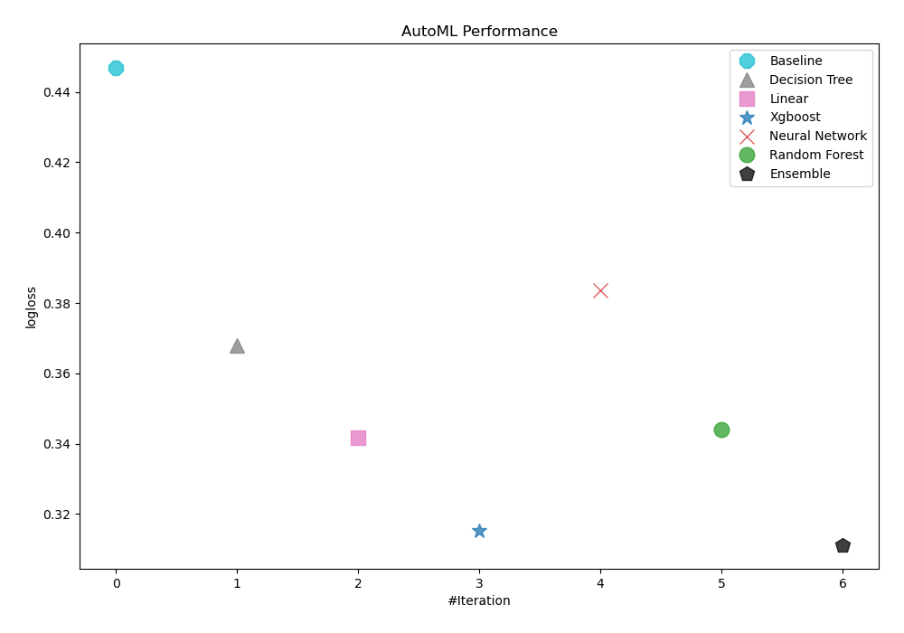
Logloss has been the performance metric used by AutoML to evaluate the performance of trained models. As a result, Ensemble was selected as the best model, as shown in the table and graph below.
| Best model | name | model_type | metric_type | metric_value | train_time |
|---|---|---|---|---|---|
| 1_Baseline | Baseline | logloss | 0.446986 | 2.26 | |
| 2_DecisionTree | Decision Tree | logloss | 0.367969 | 9.81 | |
| 3_Linear | Linear | logloss | 0.341574 | 9.69 | |
| 4_Default_Xgboost | Xgboost | logloss | 0.315124 | 11.76 | |
| 5_Default_NeuralNetwork | Neural Network | logloss | 0.383679 | 5.89 | |
| 6_Default_RandomForest | Random Forest | logloss | 0.344043 | 10.65 | |
| the best | Ensemble | Ensemble | logloss | 0.311223 | 1.65 |
Performance
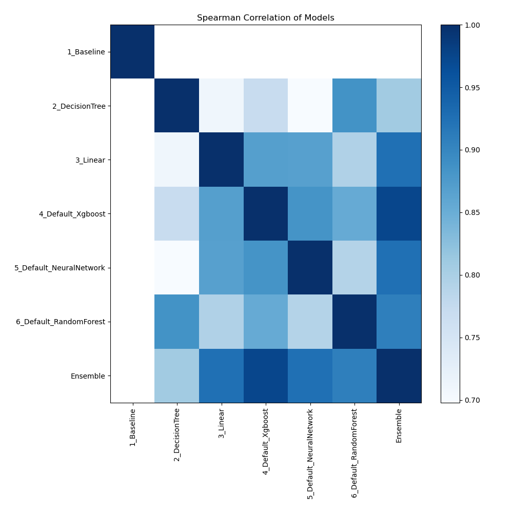
Spearman Correlation of Models
The graphic illustrates how important different features are in relation to different models. Each cell in this heatmap shows the significance of a single characteristic for a certain model, and the color intensity corresponds to the degree of significance. Lighter colors suggest lesser importance, while darker or more vivid colors indicate higher importance. By comparing the contributions of various models, this visualization aids in identifying which elements regularly contribute significantly to prediction performance and which have less of an impact.
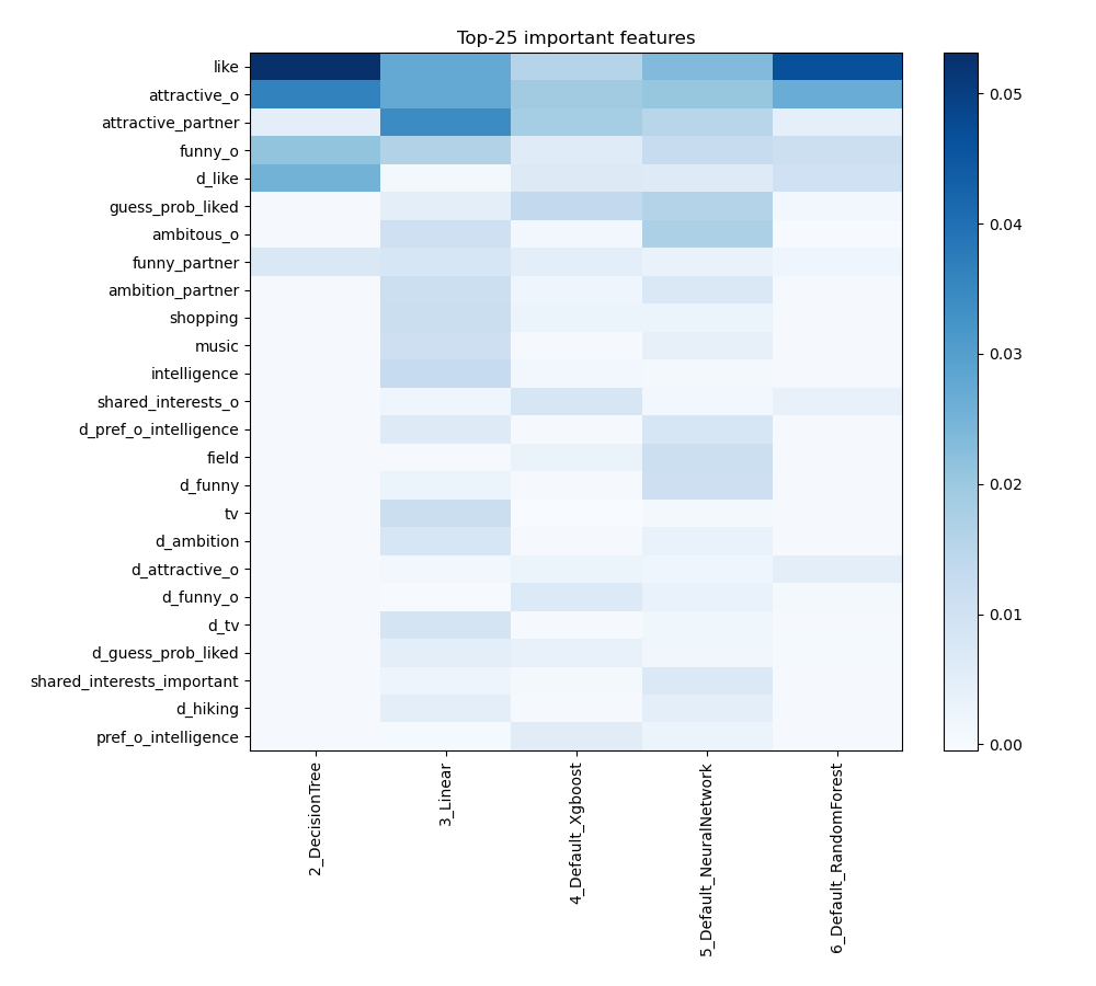
Feature Importance
The plot visualizes the significance of various features across different models. In this heatmap, each cell represents the importance of a specific feature for a particular model, with the color intensity indicating the level of importance. Darker or more intense colors signify higher importance, while lighter colors indicate lower importance. This visualization helps in comparing the contribution of features across multiple models, highlighting which features consistently play a critical role and which are less influential in predictive performance.
Install and import necessary packages
Install the packages with the command:
pip install scikit-learn, mljar-supervised
Import the packages into your code:
# import packages
from sklearn.datasets import fetch_openml
from sklearn.model_selection import train_test_split
from supervised import AutoML
from sklearn.metrics import accuracy_score
Load data
We will read data from an OpenML dataset.
# load dataset
data = fetch_openml(data_id=40536, as_frame=True)
X = data.data
y = data.target
y = y.astype("int")
# display data shape
print(f"Loaded X shape {X.shape}")
print(f"Loaded y shape {y.shape}")
# display first rows
X.head()
Loaded X shape (8378, 120)
Loaded y shape (8378,)
| has_null | wave | gender | age | age_o | d_age | d_d_age | race | race_o | samerace | ... | expected_num_interested_in_me | expected_num_matches | d_expected_happy_with_sd_people | d_expected_num_interested_in_me | d_expected_num_matches | like | guess_prob_liked | d_like | d_guess_prob_liked | met | |
|---|---|---|---|---|---|---|---|---|---|---|---|---|---|---|---|---|---|---|---|---|---|
| 0 | 0 | 1 | female | 21.0 | 27.0 | 6 | [4-6] | Asian/Pacific Islander/Asian-American | European/Caucasian-American | 0 | ... | 2.0 | 4.0 | [0-4] | [0-3] | [3-5] | 7.0 | 6.0 | [6-8] | [5-6] | 0.0 |
| 1 | 0 | 1 | female | 21.0 | 22.0 | 1 | [0-1] | Asian/Pacific Islander/Asian-American | European/Caucasian-American | 0 | ... | 2.0 | 4.0 | [0-4] | [0-3] | [3-5] | 7.0 | 5.0 | [6-8] | [5-6] | 1.0 |
| 2 | 1 | 1 | female | 21.0 | 22.0 | 1 | [0-1] | Asian/Pacific Islander/Asian-American | Asian/Pacific Islander/Asian-American | 1 | ... | 2.0 | 4.0 | [0-4] | [0-3] | [3-5] | 7.0 | NaN | [6-8] | [0-4] | 1.0 |
| 3 | 0 | 1 | female | 21.0 | 23.0 | 2 | [2-3] | Asian/Pacific Islander/Asian-American | European/Caucasian-American | 0 | ... | 2.0 | 4.0 | [0-4] | [0-3] | [3-5] | 7.0 | 6.0 | [6-8] | [5-6] | 0.0 |
| 4 | 0 | 1 | female | 21.0 | 24.0 | 3 | [2-3] | Asian/Pacific Islander/Asian-American | Latino/Hispanic American | 0 | ... | 2.0 | 4.0 | [0-4] | [0-3] | [3-5] | 6.0 | 6.0 | [6-8] | [5-6] | 0.0 |
5 rows × 120 columns
Split dataframe to train/test
To split a dataframe into train and test sets, we divide the data to create separate datasets for training and evaluating a model. This ensures we can assess the model's performance on unseen data.
# split data
X_train, X_test, y_train, y_test = train_test_split(X, y, train_size=0.90, shuffle=True, stratify=y, random_state=42)
# display data shapes
print(f"X_train shape {X_train.shape}")
print(f"X_test shape {X_test.shape}")
print(f"y_train shape {y_train.shape}")
print(f"y_test shape {y_test.shape}")
X_train shape (7540, 120)
X_test shape (838, 120)
y_train shape (7540,)
y_test shape (838,)
Fit AutoML
We need to train a model for our dataset. The fit() method will handle the model training and optimization automatically.
# create automl object
automl = AutoML(total_time_limit=300, mode="Explain")
# train automl
automl.fit(X_train, y_train)
Predict
Generate predictions using the trained AutoML model on test data.
# predict with AutoML
predictions = automl.predict(X_test)
# predicted values
print(predictions)
['1' '1' '0' ... '1' '1' '1']
Compute accuracy
We are computing the accuracy score and valid values (y_test) with our predictions.
# compute metric
metric_accuracy = accuracy_score(y_test, predictions)
print(f"Accuracy: {metric_accuracy}")
Accuracy: 0.8556085918854416
Conclusions
MLJAR AutoML simplifies the investigation of romantic preferences and relationship outcomes when used with speed dating data. It increases prediction accuracy and finds insights that traditional methods might miss by automating data processing. This results in a deeper comprehension of the complexities of dating and better decision-making in intimate partnerships. This technology has the potential to improve our understanding of love relationships and dating tactics.
See you soon👋.