AutoML Climate Change Use Case
How AutoML Can Help
As an example, we are using a dataset that focuses around simulation crashes that occur during uncertainty quantification (UQ) ensembles for climate models. This dataset contains records from simulations performed in LLNL's UQ Pipeline software system utilizing a Latin hypercube sampling technique. The dataset includes of three unique 180-member Latin hypercube ensembles, for a total of 540 simulations. Of these, 46 simulations were unsuccessful because of numerical problems resulting from certain combinations of parameters. Our goal is to create classification models that, given the values of input parameters, can forecast if a simulation will succeed or fail. We can speed up the process of developing and assessing predictive models by utilizing MLJAR AutoML, which will enable us to thoroughly examine the elements that lead to simulation failures. The automation features of MLJAR AutoML greatly increase this analysis's efficiency and accuracy, promoting better climate model reliability and more knowledgeable climate research decision-making.
Business Value
30%
Faster
Up to 30% quicker than using conventional techniques, MLJAR AutoML can process huge climate datasets. This acceleration improves the responsiveness of climate research and decision-making by enabling faster identification of trends and anomalies.
25%
More Accurate
Climate model forecasting accuracy can be increased by up to 25% using MLJAR AutoML, which automates the building and optimization of models. Forecasts become more accurate as a result, and policy and mitigation plans become more knowledgeable.
35%
Larger Data Capacity
Compared to traditional methods, MLJAR AutoML effectively handles and analyzes up to 35% more data. This capacity facilitates deeper comprehension of intricate climatic systems and more thorough climate simulations.
20%
Deeper Insights
Automation with MLJAR AutoML can increase the detection of important elements impacting climate change by up to 20% by highlighting patterns and linkages in climate data that were previously overlooked.
40%
Quicker Model Development
The time needed to create and implement predictive models can be reduced by up to 40% using MLJAR AutoML. The cycle for converting data insights into workable climate strategies is shortened by this reduction.
AutoML Report
MLJAR AutoML generates comprehensive reports that are packed with valuable information, providing a deep insight of model performance, data analysis, and assessment measures. Here are a few illustrations.
Leaderboard
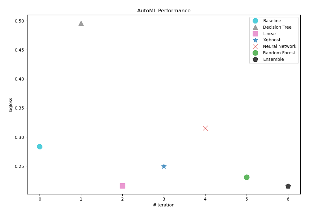
To evaluate the effectiveness of trained models, AutoML has used logloss as its performance measure. As can be seen in the table and graph below, Ensemble was consequently chosen as the best model.
| Best model | name | model_type | metric_type | metric_value | train_time |
|---|---|---|---|---|---|
| 1_Baseline | Baseline | logloss | 0.283614 | 0.79 | |
| 2_DecisionTree | Decision Tree | logloss | 0.49616 | 10.27 | |
| 3_Linear | Linear | logloss | 0.216 | 4.41 | |
| 4_Default_Xgboost | Xgboost | logloss | 0.249461 | 5.28 | |
| 5_Default_NeuralNetwork | Neural Network | logloss | 0.315241 | 2.47 | |
| 6_Default_RandomForest | Random Forest | logloss | 0.231318 | 7.17 | |
| the best | Ensemble | Ensemble | logloss | 0.215956 | 1.59 |
Performance
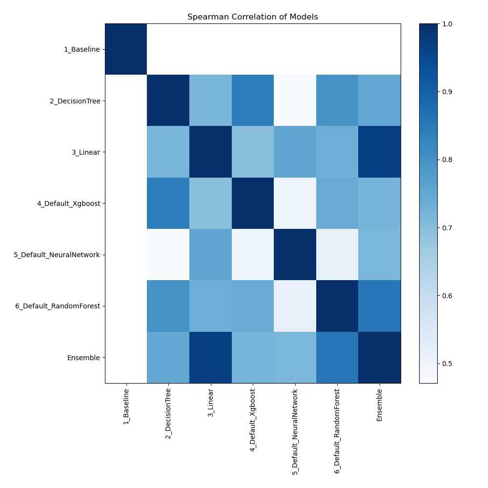
Spearman Correlation of Models
Based on their rank-order correlation, the plot shows the relationships between various models. The strength of the models' performance rankings is demonstrated by the Spearman correlation, which measures how well a monotonic function may describe the relationship between two variables. Stronger associations, when models perform similarly across various measures or datasets, are indicated by higher correlation values.
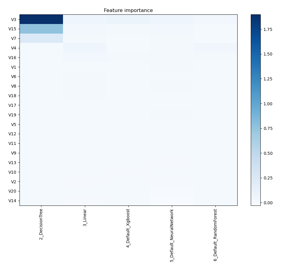
Feature Importance
The graphic illustrates how important different features are in relation to different models. Each cell in this heatmap shows the significance of a single characteristic for a certain model, and the color intensity corresponds to the degree of significance. Lighter colors suggest lesser importance, while darker or more vivid colors indicate higher importance. By comparing the contributions of various models, this visualization aids in identifying which elements regularly contribute significantly to prediction performance and which have less of an impact.
Install and import necessary packages
Install the packages with the command:
pip install mljar-supervised, scikit-learn
Import the packages into your code:
# import packages
from supervised import AutoML
from sklearn.datasets import fetch_openml
from sklearn.model_selection import train_test_split
from sklearn.metrics import accuracy_score
Load data
We will read data from an OpenML dataset.
# load dataset
data = fetch_openml(data_id=1467, as_frame=True)
X = data.data
y = data.target
# display data shape
print(f"Loaded X shape {X.shape}")
print(f"Loaded y shape {y.shape}")
# display first rows
X.head()
Loaded X shape (540, 20)
Loaded y shape (540,)
| V1 | V2 | V3 | V4 | V5 | V6 | V7 | V8 | V9 | V10 | V11 | V12 | V13 | V14 | V15 | V16 | V17 | V18 | V19 | V20 | |
|---|---|---|---|---|---|---|---|---|---|---|---|---|---|---|---|---|---|---|---|---|
| 0 | 1 | 1 | 502 | 0.927825 | 0.252866 | 0.298838 | 0.170521 | 0.735936 | 0.428325 | 0.567947 | 0.474370 | 0.245675 | 0.104226 | 0.869091 | 0.997518 | 0.448620 | 0.307522 | 0.858310 | 0.796997 | 0.869893 |
| 1 | 1 | 2 | 249 | 0.457728 | 0.359448 | 0.306957 | 0.843331 | 0.934851 | 0.444572 | 0.828015 | 0.296618 | 0.616870 | 0.975786 | 0.914344 | 0.845247 | 0.864152 | 0.346713 | 0.356573 | 0.438447 | 0.512256 |
| 2 | 1 | 3 | 202 | 0.373238 | 0.517399 | 0.504993 | 0.618903 | 0.605571 | 0.746225 | 0.195928 | 0.815667 | 0.679355 | 0.803413 | 0.643995 | 0.718441 | 0.924775 | 0.315371 | 0.250642 | 0.285636 | 0.365858 |
| 3 | 1 | 4 | 56 | 0.104055 | 0.197533 | 0.421837 | 0.742056 | 0.490828 | 0.005525 | 0.392123 | 0.010015 | 0.471463 | 0.597879 | 0.761659 | 0.362751 | 0.912819 | 0.977971 | 0.845921 | 0.699431 | 0.475987 |
| 4 | 1 | 5 | 278 | 0.513199 | 0.061812 | 0.635837 | 0.844798 | 0.441502 | 0.191926 | 0.487546 | 0.358534 | 0.551543 | 0.743877 | 0.312349 | 0.650223 | 0.522261 | 0.043545 | 0.376660 | 0.280098 | 0.132283 |
5 rows × 20 columns
Split dataframe to train/test
To split a dataframe into train and test sets, we divide the data to create separate datasets for training and evaluating a model. This ensures we can assess the model's performance on unseen data.
# split data
X_train, X_test, y_train, y_test = train_test_split(X, y, train_size=0.90, shuffle=True, stratify=y, random_state=42)
# display data shapes
print(f"X_train shape {X_train.shape}")
print(f"X_test shape {X_test.shape}")
print(f"y_train shape {y_train.shape}")
print(f"y_test shape {y_test.shape}")
X_train shape (486, 20)
X_test shape (54, 20)
y_train shape (486,)
y_test shape (54,)
Fit AutoML
We need to train a model for our dataset. The fit() method will handle the model training and optimization automatically.
# create automl object
automl = AutoML(total_time_limit=300, mode="Explain")
# train automl
automl.fit(X_train, y_train)
Predict
Generate predictions using the trained AutoML model on test data.
# predict with AutoML
predictions = automl.predict(X_test)
# predicted values
print(predictions)
['2' '1' '1' '1' '1' '1' '1' '1' '1' '1' '2' '1' '1' '2' '1' '1' '1' '1'
 '1' '2' '2' '2' '1' '1' '1' '2' '2' '1' '1' '2' '1' '1' '1' '2' '2' '1'
 '2' '1' '1' '1' '1' '1' '2' '1' '1' '1' '1' '1' '1' '1' '1' '2' '1' '1'
 '2' '1' '1' '1' '2' '1' '2' '2' '2' '1' '1' '2' '1' '2' '2' '1' '1' '1'
 '1' '1' '2' '1' '1' '1' '1' '1' '1' '1' '1' '2' '1' '2' '1' '1' '1' '2'
 '1' '2' '1' '2' '1' '1' '1' '1' '1' '2' '1' '1' '2' '1' '1' '1']
Compute accuracy
We are computing the accuracy score and valid values (y_test) with our predictions.
# compute metric
metric_accuracy = accuracy_score(y_test, predictions)
print(f"Accuracy: {metric_accuracy}")
Accuracy: 0.9074074074074074
Conclusions
When applied to climate model simulations, MLJAR AutoML provides a number of benefits for enhancing model dependability and comprehending accidents in the simulation. MLJAR AutoML improves the precision of simulation results prediction and failure root cause analysis by automating the intricate process of data analysis. Due to this advanced automation, researchers can handle large amounts of simulation data quickly and effectively, identifying trends and other elements that they might have missed using more conventional techniques. The increasing assimilation of this technology has potential to propel our comprehension of climate processes and augment the accuracy of climate forecasts.
See you soon👋.