AutoML Biology Use Case
How AutoML Can Help
MLJAR AutoML automates the use of machine learning models, which simplifies complex chemical analysis. The program helps with a number of chemical property-related activities, including determining important molecular descriptors, forecasting a compound's biodegradability, and easily and precisely assessing an impact on the environment. 1,055 samples make up the QSAR Biodegradation dataset, which also includes topological descriptors, number of atoms, and molecular weight. These characteristics, which represent the connection between molecular structure and environmental behavior, are utilized to forecast the biodegradability of substances. By automating difficult data analysis and providing accurate insights and projections that enable academics and businesses to make confident decisions and innovate, MLJAR AutoML promotes scientific and industrial growth.
Business Value
30%
Faster
Large datasets from microbiological investigations can be analyzed by MLJAR AutoML up to 30% faster than by conventional techniques, which can speed up the identification of novel microbes, genetic markers, or possible therapeutic targets. This shortens the time it takes for new discoveries to reach the market and speeds up the research cycle.
25%
More Accurate
MLJAR AutoML can increase the accuracy of predictive models used in microbiology by approximately 25% by automating the processes of model selection and adjustments. Better microbial behavior predictions, more dependable diagnoses, and more successful treatment plans are the outcomes of this.
20%
More Efficient
By optimizing processes and enhancing data management, MLJAR AutoML's integration with current laboratory information management systems (LIMS) and other data sources can increase the overall efficiency of microbiological research operations by about 20%.
30%
Lower Costs
By eliminating the requirement for specialist data science knowledge, MLJAR AutoML may result in a 30% reduction in the cost of creating and maintaining machine learning models. This makes resource allocation more efficient for microbiological labs and research organizations.
40%
More Productive
Through the automation of repetitive operations like feature engineering, data preprocessing, and model validation, MLJAR AutoML can increase researcher productivity by approximately 40%. This frees up time for more innovative and high-level strategic duties.
AutoML Report
MLJAR AutoML offers in-depth understanding of model performance, data analysis, and assessment metrics through the generation of extensive reports that are full with useful information. Here are a few examples.
Leaderboard
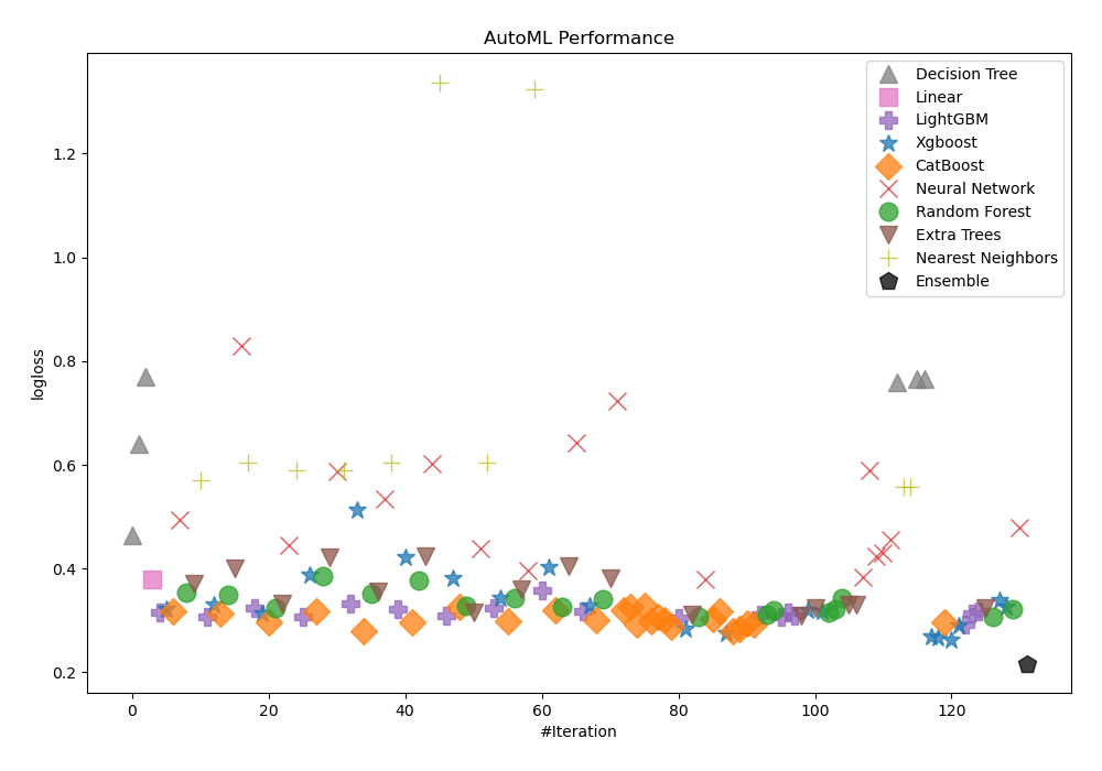
Here, Compete mode was applied to better evaluate biodegradation. It makes use of Stacked Ensemble and feature generating algorithms. For determining the effectiveness of trained models, AutoML selected logloss as its performance indicator. The table and charts below reflect its subsequent selection of Ensemble as the best model.
| Best model | name | model_type | metric_type | metric_value | train_time |
|---|---|---|---|---|---|
| 1_DecisionTree | Decision Tree | logloss | 0.465164 | 3.98 | |
| 4_Linear | Linear | logloss | 0.379504 | 3.17 | |
| 53_ExtraTrees | Extra Trees | logloss | 0.315308 | 4.1 | |
| 36_CatBoost | CatBoost | logloss | 0.298112 | 5.28 | |
| 63_NeuralNetwork | Neural Network | logloss | 0.396284 | 4.04 | |
| 31_CatBoost_GoldenFeatures | CatBoost | logloss | 0.291778 | 4.65 | |
| 34_CatBoost_KMeansFeatures | CatBoost | logloss | 0.298418 | 4.61 | |
| 33_CatBoost_RandomFeature | CatBoost | logloss | 0.300238 | 4.84 | |
| 40_RandomForest_SelectedFeatures | Random Forest | logloss | 0.306136 | 4.45 | |
| 63_NeuralNetwork_SelectedFeatures | Neural Network | logloss | 0.378618 | 4.27 | |
| 76_CatBoost_SelectedFeatures | CatBoost | logloss | 0.278526 | 4.56 | |
| 83_LightGBM | LightGBM | logloss | 0.307299 | 4.42 | |
| 86_ExtraTrees_SelectedFeatures | Extra Trees | logloss | 0.308615 | 4.85 | |
| 89_Xgboost | Xgboost | logloss | 0.318557 | 4.52 | |
| 101_NearestNeighbors | Nearest Neighbors | logloss | 0.557712 | 4.36 | |
| 108_Xgboost_SelectedFeatures | Xgboost | logloss | 0.26159 | 4.65 | |
| 110_LightGBM_SelectedFeatures | LightGBM | logloss | 0.292253 | 4.6 | |
| 114_RandomForest_SelectedFeatures | Random Forest | logloss | 0.306244 | 5.54 | |
| the best | Ensemble | Ensemble | logloss | 0.216808 | 65.36 |
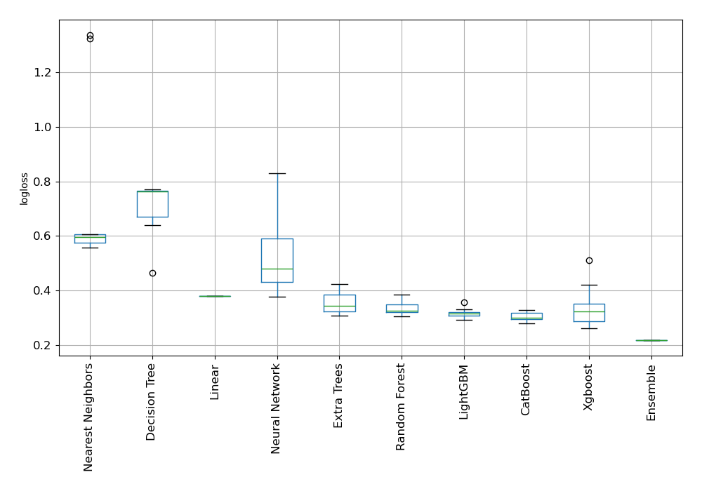
Performance
AutoML Performance Boxplot
Install and import necessary packages
Install the packages with the command:
pip install mljar-supervised, scikit-learn
Import the packages into your code:
# import packages
from supervised import AutoML
from sklearn.datasets import fetch_openml
from sklearn.model_selection import train_test_split
from sklearn.metrics import accuracy_score
Load data
We will read data from an OpenML dataset.
# load dataset
data = fetch_openml(data_id=1494, as_frame=True)
X = data.data
y = data.target
# display data shape
print(f"Loaded X shape {X.shape}")
print(f"Loaded y shape {y.shape}")
# display first rows
X.head()
Loaded X shape (1055, 41)
Loaded y shape (1055,)
| V1 | V2 | V3 | V4 | V5 | V6 | V7 | V8 | V9 | V10 | ... | V32 | V33 | V34 | V35 | V36 | V37 | V38 | V39 | V40 | V41 | |
|---|---|---|---|---|---|---|---|---|---|---|---|---|---|---|---|---|---|---|---|---|---|
| 0 | 3.919 | 2.6909 | 0 | 0 | 0 | 0 | 0 | 31.4 | 2 | 0 | ... | 0 | 0 | 0 | 0 | 2.949 | 1.591 | 0 | 7.253 | 0 | 0 |
| 1 | 4.170 | 2.1144 | 0 | 0 | 0 | 0 | 0 | 30.8 | 1 | 1 | ... | 0 | 0 | 0 | 0 | 3.315 | 1.967 | 0 | 7.257 | 0 | 0 |
| 2 | 3.932 | 3.2512 | 0 | 0 | 0 | 0 | 0 | 26.7 | 2 | 4 | ... | 0 | 0 | 0 | 1 | 3.076 | 2.417 | 0 | 7.601 | 0 | 0 |
| 3 | 3.000 | 2.7098 | 0 | 0 | 0 | 0 | 0 | 20.0 | 0 | 2 | ... | 0 | 0 | 0 | 1 | 3.046 | 5.000 | 0 | 6.690 | 0 | 0 |
| 4 | 4.236 | 3.3944 | 0 | 0 | 0 | 0 | 0 | 29.4 | 2 | 4 | ... | 0 | 0 | 0 | 0 | 3.351 | 2.405 | 0 | 8.003 | 0 | 0 |
5 rows × 41 columns
Split dataframe to train/test
To split a dataframe into train and test sets, we divide the data to create separate datasets for training and evaluating a model. This ensures we can assess the model's performance on unseen data.
# split data
X_train, X_test, y_train, y_test = train_test_split(X, y, train_size=0.90, shuffle=True, stratify=y, random_state=42)
# display data shapes
print(f"X_train shape {X_train.shape}")
print(f"X_test shape {X_test.shape}")
print(f"y_train shape {y_train.shape}")
print(f"y_test shape {y_test.shape}")
X_train shape (949, 41)
X_test shape (106, 41)
y_train shape (949,)
y_test shape (106,)
Fit AutoML
We need to train a model for our dataset. The fit() method will handle the model training and optimization automatically. As I mentioned earlier, we will use Compete mode.
# create automl object
automl = AutoML(total_time_limit=600, mode="Compete")
# train automl
automl.fit(X_train, y_train)
Predict
Generate predictions using the trained AutoML model on test data.
# predict with AutoML
predictions = automl.predict(X_test)
# predicted values
print(predictions)
['2' '1' '1' '1' '1' '1' '1' '1' '1' '1' '2' '1' '1' '2' '1' '1' '1' '1'
 '1' '2' '2' '2' '1' '1' '1' '2' '2' '1' '1' '2' '1' '1' '1' '2' '2' '1'
 '2' '1' '1' '1' '1' '1' '2' '1' '1' '1' '1' '1' '1' '1' '1' '2' '1' '1'
 '2' '1' '1' '1' '2' '1' '2' '2' '2' '1' '1' '2' '1' '2' '2' '1' '1' '1'
 '1' '1' '2' '1' '1' '1' '1' '1' '1' '1' '1' '2' '1' '2' '1' '1' '1' '2'
 '1' '2' '1' '2' '1' '1' '1' '1' '1' '2' '1' '1' '2' '1' '1' '1']
Compute accuracy
We are computing the accuracy score and valid values (y_test) with our predictions.
# compute metric
metric_accuracy = accuracy_score(y_test, predictions)
print(f"Accuracy: {metric_accuracy}")
Accuracy: 0.8301886792452831
Conclusions
There are many advantages of using MLJAR AutoML in biological research and diagnostics. By automating the examination of extensive biological and chemical data, it enables precise forecasts, early detection of biological phenomena, and the development of targeted interventions. Because AutoML manages enormous datasets efficiently, it can find patterns and insights that older approaches might miss. This technology will become more and more important in biological research and diagnostics as it develops, improving research outcomes and more.
See you soon👋.