What is Decision Tree?
Decision Tree is a hierarchical, supervised model in a tree-like shape. It supports decision making algorithms based on different variables (e.g. costs, needs, event outcomes) and its possible consequences.
It consists of:
- root node
- internal nodes
- leaf nodes
- branches
- subtrees
Decision Trees are versatile tools used for regression and classification. In addition, they are commonly used in decision analasis helping to develop best strategies. Overfitting (find out more in article) is possible in Decision Trees too. In this case pruning can be used - like in a gardening, it is trimming unnecessarry branches.
Use cases
-
Classification:
- Decision Trees are widely used for classification tasks where the goal is to assign a categorical label to input data based on their features.
- Example: Spam Email Detection - Decision Trees can classify emails as spam or non-spam based on features such as email content, sender address, and subject line. The Decision Tree learns rules to differentiate between spam and non-spam emails, allowing for effective filtering of unwanted messages.
-
Regression:
- Decision Trees can also be used for regression tasks where the goal is to predict a continuous target variable based on input features.
- Example: House Price Prediction - Decision Trees can predict the selling price of a house based on features such as size, location, number of bedrooms, and amenities. The Decision Tree learns patterns in the data to make accurate price predictions for new properties.
-
Feature Selection:
- Decision Trees can be used for feature selection, where the most informative features are identified based on their importance in the decision-making process.
- Example: Customer Segmentation - Decision Trees can help identify the most relevant features for segmenting customers into different groups based on their purchasing behavior, demographics, and preferences. By focusing on the most informative features, businesses can tailor marketing strategies and improve customer engagement.
Decision Tree structure
You can also think about Decision Tree diagram as a flowchart helping to visualize plans or predictions.
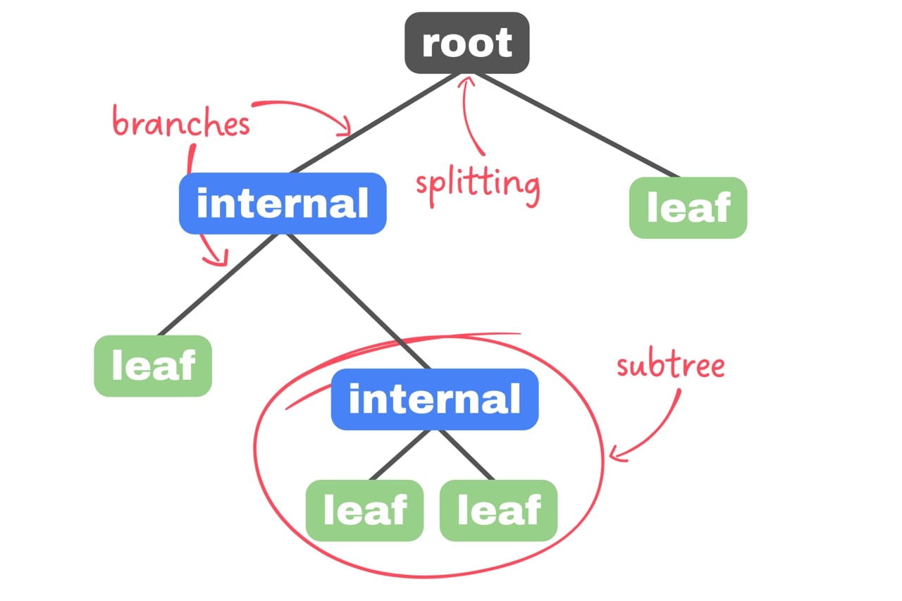
Our starting point is root node, single one node with only outgoing branches. It’s connected to internal/decision nodes. Each of those nodes must make a decision from given dataset. From every node comes out two branches, representing possible choices. The ending points of Decision Tree are leaf nodes – resolutions of integral nodes making decisions. Every leaf node has only one incoming branch and they represent all possible outcomes for our data. Possible is for Decision Tree to contain similar leafs in different subtrees.
Best node-splitting functions and their use
Decision Tree algorithms use many different methods to split nodes. It is a fundamental concept in those algorithms trying to achieve pure nodes (these nodes contain only one homogenous class – ergo, takes into consideration part of data that no other node does). Most popular, evaluating the quality of each test condition splitting methods are:
-
Entropy
- It’s a measure of impurity in dataset that ranges from 0 to 1 with too complex formula. The more elements evenly distributed among classes, the higher entropy. The more entropy, the more uncertain data. Do we want to have uncertain nodes? Not really. Machine learning goal in wider understanding is to make uncertain things clearer for us so we can split this uncertain node, however we don’t know how splitting a node influences certainty of parent node.
-
Gini impurity
- Other metric used in Decision Trees (sometimes named Gini index) and alternative to regression. It grades - 0 is fully organized, 0.5 is totally mixed - nodes to splitting based on organization of dataset so lower values are preferable.
-
Information gain
- It represents weight of the split, difference in entropy or Gini index before and after split. Information gain has tangled algorithm using both metrics. To properly train Decision Tree information gain is used to find its highest values and split it making continues subtrees. Creating algorithm in training focuses on prefferably single variables in dataset having most influance on result and positioning those splits higher in hierarchy of the tree.
Gini impurity is easier to compute than Entropy (summing and sqering instead of logarythms and multiplacations), so for time efficiency Gini inex is usually chosen over entrophy for Decision Tree algorithm.
History of Decision Tree
Decision Trees were first proposed by Arthur L. Samuel in 1959 while he was at IBM. However, it was not until the 1980s and 1990s that Decision Trees gained significant popularity and were further developed by researchers such as Ross Quinlan, J. Ross Quinlan, and others.
Quinlan's work on Decision Trees, particularly his development of the ID3 (Iterative Dichotomiser 3) algorithm in the 1980s, played a crucial role in advancing the field of machine learning and Decision Tree-based methods. Quinlan's subsequent algorithms, such as C4.5 and its successor C5.0, further refined and improved Decision Tree algorithms, making them widely used in various applications.
How to use it?
Here's an example of Python code that uses scikit-learn's datasets module to load the Iris dataset, splits it into training and testing sets, and trains a DecisionTreeClassifier on it:
from sklearn.datasets import load_iris
from sklearn.model_selection import train_test_split
from sklearn.tree import DecisionTreeClassifier
from sklearn.metrics import accuracy_score

# Load the Iris dataset
iris = load_iris()
X = iris.data  # Features
y = iris.target  # Target variable

# Split the dataset into training and testing sets
X_train, X_test, y_train, y_test = train_test_split(X, y, test_size=0.2, random_state=42)

# Initialize Decision Tree classifier
tree_classifier = DecisionTreeClassifier()

# Train the classifier on the training data
tree_classifier.fit(X_train, y_train)

# Make predictions on the test data
predictions = tree_classifier.predict(X_test)

# Evaluate the model
accuracy = accuracy_score(y_test, predictions)
print("Accuracy:", accuracy)
In this code:
- We import the
load_irisfunction from sklearn.datasets to load the Iris dataset. - We split the dataset into training and testing sets using the
train_test_splitfunction from sklearn.model_selection. - We import class from sklearn.tree to initialize a Decission Tree classifier.
- We import the
accuracy_score()function from sklearn.metrics to evaluate the model's accuracy. - We train the Decision Tree classifier on the training data using the fit method.
- We make predictions on the test data using the predict method.
- Finally, we evaluate the model's performance using the accuracy score.
Pros and cons
Decision Trees have wide usage but are usually outperformed by more precise algorithms. However they shine most notably in data science and data-mining.
-
Advantages:
- Human readability - Decision Tree diagrams are not difficult to read, unlike some other models.
- Features selection - Decision Tree provides feedback about feature importance.
- Quick training - binary tree architecture of Decision Trees make them require little to no training.
-
Disadvantages:
- Butterfly effect - small changes in dataset can "mutate" decission tree to very different structure.
- Underfitting - Decision Trees sometimes can't handle complex dependencies between data.
- Need of pruning - Decision Trees easily overfit in the face of new data.
Literature
Decision Trees are wide and deep subject but we can offer some insight where to start your adventure:
- C4.5: Programs for Machine Learning" by J. Ross Quinlan - possibly no one finds it strange to see this name on first place. This book by J. Ross Quinlan, the creator of the C4.5 algorithm, provides a comprehensive overview of Decision Trees and their application in machine learning. It covers the theory behind Decision Trees, the C4.5 algorithm, and practical implementation details. The book also includes case studies and examples to illustrate the concepts discussed.
- A comparative study of Decision Tree ID3 and C4.5 from Sultan Moulay Slimane University - for those interested in getting accustomed with changes to Decision Tree models and changes made to them.
Conclusions
Decision Trees are powerful and versatile machine learning algorithms that are widely used for bothclassification and regression tasks.
Overall, Decision Trees are popular due to their simplicity, interpretability, and ability to handle various types of data and tasks. However, they require careful tuning to avoid overfitting and may not always perform as well as more complex algorithms on certain datasets. Nonetheless, they remain a valuable tool in the machine learning toolkit.